

Denoising Diffusion Probabilistic Models (DDPM)
The goal: learn the distribution of images, so you can draw new ones from it.
Two obstacles sit between us and the goal.
-
A 32×32×3 image is 3,072 numbers. Writing down \(p(x)\) directly means an integral function over all of \(\mathbb{R}^{3072}\) and a normalization we can never compute, and it also ignores what makes an image an image. Pixels. Unlike us, pixels like their neighbours. so its important to capture those dependencies.
-
A model that assigns good probability to an image is not automatically one you can produce images from. Those are two different demands, and a method can pass one and fail the other.
VAE and GAN preceed this way of trying to solve these issues. VAE sidesteps the integral by introducing a latent \(z\), but then forces everything about a 256×256 image through a vector that is lower-dimensional by design. That bottleneck throws away precisely the high-frequency detail that makes an image look real, so reconstructions come out blurry. A GAN refuses the bottleneck and gets sharp samples, but with no likelihood to optimize it trains by an adversarial game that is unstable and prone to mode collapse.
So I try to think about what the authors needed then wasn’t just a cleverer model. I like to think they wanted an objective they could evaluate. Something whose gradient they could compute on a fixed budget, with no adversarial game and no narrow neck. Now how they went from this need to the diffusion process of corrupt the image in many small steps until only noise is left, then learn to undo one step at a time. Make the corruption simple enough to be invertible in closed form, and learn only the part that isn’t.. this part, well some researchers are gifted in that sense I guess.
I wanted to deep dive into this paper as all the other diffusion papers kind of pull from this, so if I can understand this deeply, I’ll have the intuition to understand the others. so here goes. Also note, big chunks of this are from the paper. I’m not claiming this is originalk. I’m just trying to learn things and releasing my notes so I can reference back these later on.
Legend.
- \(q\) is forward: the fixed process that destroys the image.
- \(p\) is backward: the model that undoes it, written \(p_\theta\) whenever a parameter matters and plain \(p\) when it doesn’t.
- A subscript is the timestep: \(x_0\) is the clean image, \(x_t\) is the image after \(t\) steps of noise, \(x_T\) is pure noise.
1. The problem
Concretely, the thing we would have to compute is
\[p_\theta(x_0) = \int p_\theta(x_{0:T})\, dx_{1:T}\]an ordinary likelihood, factored over \(T\) extra variables. The integral is over \(x_1, \dots, x_T\), and if we get to choose what those variables are, we can choose a process whose terms we can evaluate. §2 makes that choice.
The design constraint is sharp. We need each term to be cheap to compute, and we need the product over \(T\) steps to stay tractable rather than collapsing into a new intractable integral. Whichever process satisfies both is the one we are allowed to build.
The forward process walks the image through a chain, \(x_0 \to x_1 \to \cdots \to x_T\), and because it is Markov, the probability of a whole trajectory is just the product of the individual transitions:
\[q(x_{1:T}\mid x_0) = \prod_{t=1}^{T} q(x_t\mid x_{t-1})\]Each factor is one small, simple step. Multiplying simple pieces is perfectly manageable.
But multiplying simple pieces does not guarantee the result is simple. If each transition had some arbitrary nonlinear form, then to get the distribution of a later state you would have to integrate out every intermediate one:
\[q(x_2\mid x_0) = \int q(x_2\mid x_1)\,q(x_1\mid x_0)\,dx_1\]and for three steps,
\[q(x_3\mid x_0) = \iint q(x_3\mid x_2)\,q(x_2\mid x_1)\,q(x_1\mid x_0)\,dx_1\,dx_2\]Every extra step adds another integration over a space as large as the image. That nest of integrals is what “intractable” means here: not merely big, but with no usable analytical solution and too expensive to approximate numerically. A method built this way would be dead on arrival, because training needs \(q(x_t\mid x_0)\) for arbitrary \(t\) at every single step.
Gaussian transitions are what avoid it. If each step is
\[q(x_t\mid x_{t-1}) = \mathcal{N}\!\left(x_t; \sqrt{1-\beta_t}\,x_{t-1}, \beta_t I\right)\]then the composition of Gaussians is still Gaussian, so the whole nested integral collapses to a single closed form. With \(\alpha_t = 1-\beta_t\) and \(\bar{\alpha}_t = \prod_{s=1}^{t}\alpha_s\):
\[q(x_t\mid x_0) = \mathcal{N}\!\left(x_t; \sqrt{\bar{\alpha}_t}\,x_0, (1-\bar{\alpha}_t)I\right)\]so we can jump straight to any timestep,
\[x_t = \sqrt{\bar{\alpha}_t}\,x_0 + \sqrt{1-\bar{\alpha}_t}\,\epsilon, \qquad \epsilon \sim \mathcal{N}(0, I)\]no simulation of \(x_1,\dots,x_{t-1}\) required. That is §2.2’s induction, and it is the reason training is cheap.
This is whats the simple beauty of this appraoch. A forward process simple enough that everything downstream has a closed form. Gorgeous.
2. The move
destroy structure, learn to restore it
2.1 Notation
- \(\beta_t\) -> the variance of one forward step. The sequence \(\beta_1,\dots,\beta_T\) is a fixed schedule, a hyperparameter, not something learned.
- \(\alpha_t := 1 - \beta_t\) -> how much signal survives one forward step.
- \(\bar{\alpha}_t := \prod_{s=1}^t \alpha_s\) -> how much survives from \(t=0\) to \(t\).
The paper uses \(T = 1000\) and \(\beta_t\) linear from \(10^{-4}\) to \(0.02\), so \(\bar{\alpha}_T\) is tiny by the end.
In the code every one of these is a precomputed array, indexed by \(t\) (sqrt_alphas_cumprod, sqrt_one_minus_alphas_cumprod, posterior_variance, posterior_mean_coef1/2, all built once in __init__ (lines 64–81)).
The two chains are:
\[q(x_{1:T}\mid x_0) := \prod_{t=1}^T q(x_t\mid x_{t-1}), \qquad q(x_t\mid x_{t-1}) := \mathcal{N}(x_t; \sqrt{1-\beta_t}\,x_{t-1}, \beta_t I)\] \[p_\theta(x_{0:T}) := p(x_T)\prod_{t=1}^T p_\theta(x_{t-1}\mid x_t), \qquad p_\theta(x_{t-1}\mid x_t) := \mathcal{N}(x_{t-1}; \mu_\theta(x_t, t), \Sigma_\theta(x_t, t))\]These are Eqs. (1) and (2) of the paper, with \(p(x_T) = \mathcal{N}(x_T; 0, I)\).
The core idea is that noise to image in one shot is hopeless, but a single denoising step from \(x_t\) to \(x_{t-1}\) is easy enough to learn. Do it a thousand times and an image falls out. Beautiful.
2.2 forward
We want \(q(x_t\mid x_0)\): where an image ends up after \(t\) steps of noising. Simulating \(t\) steps answers it, but there is a direct formula.
Claim: \(q(x_t\mid x_0) = \mathcal{N}(x_t; \sqrt{\bar{\alpha}_t}\,x_0, (1-\bar{\alpha}_t)I)\).
Proof by induction.
Base case \(t=1\): by definition \(q(x_1\mid x_0) = \mathcal{N}(x_1; \sqrt{\alpha_1}\,x_0, \beta_1 I)\), and since \(\bar{\alpha}_1 = \alpha_1\) and \(\beta_1 = 1-\alpha_1\), this is \(\mathcal{N}(x_1; \sqrt{\bar{\alpha}_1}\,x_0, (1-\bar{\alpha}_1)I)\). ✓
Inductive step. Assume \(q(x_{t-1}\mid x_0) = \mathcal{N}(x_{t-1}; \sqrt{\bar{\alpha}_{t-1}}\,x_0, (1-\bar{\alpha}_{t-1})I)\), and write both steps as reparameterized samples:
\[x_{t-1} = \sqrt{\bar{\alpha}_{t-1}}\,x_0 + \sqrt{1-\bar{\alpha}_{t-1}}\,\epsilon_{t-1}, \qquad \epsilon_{t-1} \sim \mathcal{N}(0, I)\] \[x_t = \sqrt{\alpha_t}\,x_{t-1} + \sqrt{\beta_t}\,\epsilon_t, \qquad \epsilon_t \sim \mathcal{N}(0, I)\]Substituting the first into the second:
\[x_t = \sqrt{\alpha_t}\left(\sqrt{\bar{\alpha}_{t-1}}\,x_0 + \sqrt{1-\bar{\alpha}_{t-1}}\,\epsilon_{t-1}\right) + \sqrt{\beta_t}\,\epsilon_t\] \[= \sqrt{\alpha_t\bar{\alpha}_{t-1}}\,x_0 + \sqrt{\alpha_t(1-\bar{\alpha}_{t-1})}\,\epsilon_{t-1} + \sqrt{\beta_t}\,\epsilon_t\]The last two terms are independent Gaussians, so their sum is Gaussian with the variances added:
\[\sqrt{\alpha_t(1-\bar{\alpha}_{t-1})}\,\epsilon_{t-1} + \sqrt{\beta_t}\,\epsilon_t \sim \mathcal{N}\!\left(0, \left[\alpha_t(1-\bar{\alpha}_{t-1}) + \beta_t\right]I\right)\]Simplify the variance, using \(\beta_t = 1-\alpha_t\):
\[\alpha_t(1-\bar{\alpha}_{t-1}) + \beta_t = \alpha_t - \alpha_t\bar{\alpha}_{t-1} + 1 - \alpha_t = 1 - \alpha_t\bar{\alpha}_{t-1} = 1 - \bar{\alpha}_t\]Also \(\sqrt{\alpha_t\bar{\alpha}_{t-1}} = \sqrt{\bar{\alpha}_t}\). Therefore \(q(x_t\mid x_0) = \mathcal{N}(x_t; \sqrt{\bar{\alpha}_t}\,x_0, (1-\bar{\alpha}_t)I)\). \(\blacksquare\)
This is Eq. (4), and it gives a very important identity —> the reparameterization:
\[x_t = \sqrt{\bar{\alpha}_t}\,x_0 + \sqrt{1-\bar{\alpha}_t}\,\epsilon, \qquad \epsilon \sim \mathcal{N}(0, I)\]At each \(t\) the two coefficients do opposite jobs, and together they are why this collapses so cleanly:
- \(\sqrt{\bar{\alpha}_t}\) - the signal coefficient: how much of the original image is still there, shrinking from 1 toward 0.
- \(\sqrt{1-\bar{\alpha}_t}\) - the noise coefficient: the standard deviation of the accumulated noise, growing from 0 toward 1.
Because of this paramterized formula for the forward process, we can literally jump to any noise level instead of simulating the chain. Sample a random \(t\), corrupt the image directly, take a gradient step. That is what makes training cheap, and it is six lines of code: q_sample (lines 101–111) is literally sqrt_alphas_cumprod[t] * x_0 + sqrt_one_minus_alphas_cumprod[t] * noise.
2.3 reverse
The reverse chain is Eq. (1): start at \(p(x_T) = \mathcal{N}(0,I)\), then for \(t = T,\dots,1\) sample \(x_{t-1} \sim p_\theta(x_{t-1}\mid x_t) , \qquad p_\theta(x_{t-1}\mid x_t) = \mathcal{N}(x_{t-1}; \mu_\theta(x_t,t), \Sigma_\theta(x_t,t))\).
Why assume the reverse steps are Gaussian? My AI says::: When each \(\beta_t\) is small, the forward process takes steps so tiny that its transition kernel is barely different from the reverse one, and both land in the same functional family (Sohl-Dickstein et al., 2015). A small Gaussian step is approximately invertible by another Gaussian step, so assuming Gaussian reverse conditionals and letting the network learn their means is reasonable. The assumption is not exact; it becomes one in the continuous-time limit, which is where the theory is formally stated. I haven’t delved into the proof for this. maybe I’ll return to this some day. for now, I want to focus on the application.
The mean is learned. The covariance is fixed to a constant schedule, \(\Sigma_\theta(x_t,t) = \sigma_t^2 I\), with two candidate choices:
- \(\sigma_t^2 = \beta_t\): the variance of a single forward step. Optimal when \(x_0 \sim \mathcal{N}(0,I)\).
- \(\sigma_t^2 = \tilde{\beta}_t\): the variance of the forward posterior \(q(x_{t-1}\mid x_t, x_0)\) (derived in §4.2). Optimal when \(x_0\) is fixed at one point.
The paper tried both and got similar results; they are the two extremes, upper and lower bounds on reverse process entropy for data with coordinatewise unit variance. So the covariance is never predicted, and the only learned quantity is the mean \(\mu_\theta(x_t,t)\).
in code - AI generated
p_mean_variance has three modes (lines 133–148), and the point of all of them is that the network is never asked about the variance.
The two fixed modes. With model_var_type set to 'fixedlarge' or 'fixedsmall', the variance is a number looked up from a precomputed array:
'fixedlarge'usesself.betas, i.e. \(\sigma_t^2 = \beta_t\).'fixedsmall'usesself.posterior_variance, i.e. \(\sigma_t^2 = \tilde{\beta}_t\).
The variance array for fixedlarge is not plain betas: it is np.append(self.posterior_variance[1], self.betas[1:]), which replaces the first slot. That slot is \(t=0\), where the clean image sits, and the patch exists because a raw \(\beta\) there gives the wrong decoder behaviour - the code’s own comment says it is “to get a better decoder log likelihood”. Line 79 does the same to the log array, overwriting its first entry so np.log never meets the zero this schedule produces at that position. Then _extract (lines 84–93) indexes those arrays at the batch’s timesteps and reshapes them to [B,1,1,1,C], so a 1-D schedule broadcasts against a whole batch of images.
Why a log array at all - and where it meets Eq. (5)
This is the link that is easy to miss. The bound of Eq. (5) is built out of per-step KLs:
\[L = \mathbb{E}_q\Big[L_T + \sum_{t=2}^{T} L_{t-1} + L_0\Big], \qquad L_{t-1} = D_{\text{KL}}\big(q(x_{t-1}\mid x_t, x_0) \,\|\, p_\theta(x_{t-1}\mid x_t)\big)\]So the quantity the code has to compute is a KL between two Gaussians whose covariance is fixed. That is the only reason the variance appears in the loss at all: it is an argument of the KL. And §4.3’s variance-form KL,
\[D_{\text{KL}} = \frac{1}{2}\left[d\log\frac{\sigma_2^2}{\sigma_1^2} - d + \frac{d\sigma_1^2}{\sigma_2^2}\right] + \frac{\|\mu_1-\mu_2\|^2}{2\sigma_2^2}\]depends on the variances only through a log and two ratios - a log of a ratio, and an inverse variance. With \(\texttt{logvar} = \log\sigma^2\) those three pieces are trivial:
\[\log\frac{\sigma_2^2}{\sigma_1^2} = \texttt{logvar}_2 - \texttt{logvar}_1, \qquad \frac{\sigma_1^2}{\sigma_2^2} = e^{\texttt{logvar}_1-\texttt{logvar}_2}, \qquad \frac{1}{\sigma_2^2} = e^{-\texttt{logvar}_2}\]which is exactly what normal_kl (lines 8–13) computes:
0.5 * (-1.0 + logvar2 - logvar1 + tf.exp(logvar1 - logvar2)
       + tf.squared_difference(mean1, mean2) * tf.exp(-logvar2))
Read it against the equation term for term: logvar2 - logvar1 is the log term, exp(logvar1 - logvar2) is \(\sigma_1^2/\sigma_2^2\), exp(-logvar2) is \(1/\sigma_2^2\), and -1.0 is the \(-d\) at one pixel. Same function, rearranged; I checked the two forms agree numerically on random inputs.
So the variance is carried as a log for the same reason it is in the loss at all - it is an argument to the KL, and the KL only ever asks for \(\log\sigma^2\) and \(1/\sigma^2\). The code keeps the plain variance too because two places in the loss are not in log form, both of them about the mean: the \(1/(2\sigma_t^2)\) weight on \(\|\tilde{\mu}_t - \mu_\theta\|^2\) in Eq. (8), and the inverse variance inside that norm.
The third mode. 'learned' is the one real alternative. The network’s output is doubled - it is built with out_ch = C*2 if model_var_type == 'learned' else C - and split in half: one half is the mean, the other is \(\log\sigma_t^2\) per pixel, exponentiated to give the variance (lines 134–137).
That is DDPM’s own attempt at a learned variance, and it is not what iDDPM does. Predicting \(\log\sigma_t^2\) directly is the thing that proved unstable, which is why the default is fixedlarge. iDDPM instead predicts a weight \(v\) between the two bounds and interpolates in log space,
so the result cannot leave the valid range no matter what the network outputs.
3. The bound
§1 said \(p_\theta(x_0) = \int p_\theta(x_{0:T})\,dx_{1:T}\) is uncomputable. Luckily we can bypass this with importance sampling, sitting on the shoulder of math giants.
Importance sampling is the standard way around such problems. If you cannot sample from the distribution you care about, sample from one you can and reweight each sample by how much the two disagree. For any \(q\) that is nonzero wherever \(p_\theta\) is,
\[\int p_\theta(x_{0:T})\,f(x_{0:T})\,dx_{1:T} = \int q(x_{1:T}\mid x_0)\,\underbrace{\frac{p_\theta(x_{0:T})}{q(x_{1:T}\mid x_0)}}_{\text{importance weight}}\,f(x_{0:T})\,dx_{1:T} = \mathbb{E}_q\!\left[\frac{p_\theta(x_{0:T})}{q(x_{1:T}\mid x_0)}\,f\right]\]right-hand side is now an expectation under \(q\), and \(q\) is ours to choose. Here it will be the fixed forward process, which we can sample from trivially. Set \(f \equiv 1\) and the average weight is exactly the density we wanted:
\[\log p_\theta(x_0) = \log \mathbb{E}_q\!\left[\frac{p_\theta(x_{0:T})}{q(x_{1:T}\mid x_0)}\right]\]Jensen
Why not just estimate that expectation by sampling and be done? Because we need \(\log p_\theta(x_0)\), per datapoint and differentiable.
\(p_\theta(x_0)\) is a density, usually astronomically small, so a Monte Carlo average over a handful of weights is a hopeless estimate and taking the log of that noise is worse. Jensen lets the log go inside. Since \(\log\) is concave, \(f(\mathbb{E}[X]) \geq \mathbb{E}[f(X)]\):
\[\log p_\theta(x_0) = \log \mathbb{E}_q\!\left[\frac{p_\theta(x_{0:T})}{q(x_{1:T}\mid x_0)}\right] \geq \mathbb{E}_q\!\left[\log \frac{p_\theta(x_{0:T})}{q(x_{1:T}\mid x_0)}\right]\]and this is what makes the objective computable. By Eqs. (1) and (2) the argument is a product of \(T\) terms; the log turns it into a sum of \(T\) terms, one log-ratio per step. A product over the chain is untouchable, but a sum we can unroll.
The price is that it is no longer an equality. So what is the gap?
gap = KL
Take the difference and write \(p_\theta(x_{0:T}) = p_\theta(x_0)\,p_\theta(x_{1:T}\mid x_0)\):
\[\log p_\theta(x_0) - \mathbb{E}_q\!\left[\log \frac{p_\theta(x_{0:T})}{q(x_{1:T}\mid x_0)}\right] = \log p_\theta(x_0) - \mathbb{E}_q\!\left[\log p_\theta(x_0) + \log \frac{p_\theta(x_{1:T}\mid x_0)}{q(x_{1:T}\mid x_0)}\right]\]The \(\log p_\theta(x_0)\) term is constant under \(\mathbb{E}_q\).
\(x_0\) is observed, not sampled, hence the two copies cancel:
\[= -\mathbb{E}_q\!\left[\log \frac{p_\theta(x_{1:T}\mid x_0)}{q(x_{1:T}\mid x_0)}\right] = D_{\text{KL}}\!\left(q(x_{1:T}\mid x_0)\,\|\,p_\theta(x_{1:T}\mid x_0)\right)\]so imagine A≥B, and G is the gap diff between A & B. then A = B+G essentially we now have what the eq 5 which $logp_{\theta}(x_0)=B+G$, B being the elbo expression from before and the G being the KL gap we just found. Hence:
\[\log p_\theta(x_0) = \underbrace{\mathbb{E}_q\!\left[\log \frac{p_\theta(x_{0:T})}{q(x_{1:T}\mid x_0)}\right]}_{\text{ELBO}} + \underbrace{D_{\text{KL}}\!\left(q(x_{1:T}\mid x_0)\,\|\,p_\theta(x_{1:T}\mid x_0)\right)}_{\ \geq\, 0}\]So the objective is forced: maximize the bound, and the bound’s job is to push \(p_\theta\) onto \(q\). The ML convention is to minimize the negative log-likelihood, so multiply the identity by \(-1\). Flipping the sign reverses the inequality, because subtracting a non-negative KL can only make the number smaller:
\[\mathbb{E}\left[-\log p_\theta(x_0)\right] \leq \mathbb{E}_q\!\left[-\log \frac{p_\theta(x_{0:T})}{q(x_{1:T}\mid x_0)}\right] =: L\]So \(L = -\text{ELBO}\): an upper bound on the NLL, and minimizing it is the same act as maximizing the ELBO.
The two forms of Eq. (3)
Eq. (3) in the paper writes \(L\) twice. The first is the form above. The second comes from substituting the two chain definitions, Eqs. (1) and (2):
\[p_\theta(x_{0:T}) = p(x_T)\prod_{t=1}^{T}p_\theta(x_{t-1}\mid x_t), \qquad q(x_{1:T}\mid x_0) = \prod_{t=1}^{T}q(x_t\mid x_{t-1})\]The numerator has \(T+1\) factors and the denominator has \(T\), indexed compatibly, so they pair off one for one. Each \(p_\theta(x_{t-1}\mid x_t)\) over its matching \(q(x_t\mid x_{t-1})\):
\[\frac{p_\theta(x_{0:T})}{q(x_{1:T}\mid x_0)} = p(x_T)\prod_{t=1}^{T}\frac{p_\theta(x_{t-1}\mid x_t)}{q(x_t\mid x_{t-1})}\]The lone \(p(x_T)\) is the factor with no partner: it is the start of the reverse chain, and the forward chain has nothing corresponding to it. Taking \(-\log\) and using log-of-a-product-is-sum-of-logs gives the second form,
\[L = \mathbb{E}_q\!\left[-\log p(x_T) - \sum_{t\ge 1} \log \frac{p_\theta(x_{t-1}\mid x_t)}{q(x_t\mid x_{t-1})}\right]\]That second form is the one we can compute: \(T\) separate terms instead of one uncomputable lump, each a log-ratio between the reverse and forward transition at a single step, plus one term for the prior.
4. Derivations
\(L\) is one lump over the whole chain. Unrolling the products in Eqs. (1) and (2) splits it into per-step pieces, all Gaussian KLs.
4.1 Unrolling Eq. (3) to Eq. (5)
Start from the definition of \(L\) and expand both products:
\[L = \mathbb{E}_q\!\left[-\log p(x_T) - \sum_{t=1}^T \log \frac{p_\theta(x_{t-1}\mid x_t)}{q(x_t\mid x_{t-1})}\right]\]Separate the \(t=1\) term:
\[L = \mathbb{E}_q\!\left[-\log p(x_T) - \sum_{t=2}^T \log \frac{p_\theta(x_{t-1}\mid x_t)}{q(x_t\mid x_{t-1})} - \log \frac{p_\theta(x_0\mid x_1)}{q(x_1\mid x_0)}\right]\]Now the key step. Bayes’ rule on the forward process:
\[q(x_t\mid x_{t-1}) = \frac{q(x_{t-1}\mid x_t, x_0)\,q(x_t\mid x_0)}{q(x_{t-1}\mid x_0)}\]This holds because \(q(x_t\mid x_{t-1}, x_0) = q(x_t\mid x_{t-1})\) as the forward chain is Markovian, so conditioning on the clean image adds nothing once you know \(x_{t-1}\). Substituting:
\[\log \frac{p_\theta(x_{t-1}\mid x_t)}{q(x_t\mid x_{t-1})} = \log \frac{p_\theta(x_{t-1}\mid x_t)}{q(x_{t-1}\mid x_t, x_0)} - \log q(x_t\mid x_0) + \log q(x_{t-1}\mid x_0)\]Summing over \(t = 2,\dots,T\), the last two terms telescope:
\[-\sum_{t=2}^T \log q(x_t\mid x_0) + \sum_{t=2}^T \log q(x_{t-1}\mid x_0) = -\log q(x_T\mid x_0) + \log q(x_1\mid x_0)\]Putting it back together:
\[L = \mathbb{E}_q\!\left[-\log \frac{p(x_T)}{q(x_T\mid x_0)} - \sum_{t=2}^T \log \frac{p_\theta(x_{t-1}\mid x_t)}{q(x_{t-1}\mid x_t, x_0)} - \log p_\theta(x_0\mid x_1)\right]\]which is three groups of terms, written as divergences:
\[L = \mathbb{E}_q\Big[\underbrace{D_{\text{KL}}(q(x_T\mid x_0)\,\|\,p(x_T))}_{L_T} + \sum_{t=2}^T \underbrace{D_{\text{KL}}(q(x_{t-1}\mid x_t, x_0)\,\|\,p_\theta(x_{t-1}\mid x_t))}_{L_{t-1}} + \underbrace{\left(-\log p_\theta(x_0\mid x_1)\right)}_{L_0}\Big]\]That is Eq. (5). Term by term for intuition:
- \(L_T\): how far the fully noised image is from the prior. The forward process has no parameters and \(p(x_T) = \mathcal{N}(0,I)\), so this is constant, gets no gradient, and is ignored. In practice it is about \(10^{-5}\) bits/dim, which is why the schedule is chosen as it is.
- \(L_{t-1}\): compares the true forward posterior \(q(x_{t-1}\mid x_t, x_0)\) (what noising actually did) against the learned reverse step \(p_\theta(x_{t-1}\mid x_t)\). Two Gaussians, so it has a closed form. This is the term that trains the denoiser.
- \(L_0\): how much likelihood the model gives the clean image given \(x_1\).
One computational note that matters: the bound’s KLs run in the direction \(D_{\text{KL}}(q \,\|\, p_\theta)\) - the expectation is under the fixed forward process, so the terms are cheap and low-variance and need no reweighting.
Every term here needs \(q(x_{t-1}\mid x_t, x_0)\)
4.2 The forward process posterior \(q(x_{t-1}\mid x_t, x_0)\)
We want the distribution of the slightly cleaner image given the noisier one and the original. Knowing \(x_0\) is what makes this tractable; the network will not have \(x_0\), and §5 fixes that.
Step 1: Bayes’ rule
\[q(x_{t-1}\mid x_t, x_0) = \frac{q(x_t\mid x_{t-1}, x_0)\,q(x_{t-1}\mid x_0)}{q(x_t\mid x_0)} = \frac{q(x_t\mid x_{t-1})\,q(x_{t-1}\mid x_0)}{q(x_t\mid x_0)}\]using the Markov property again. All three pieces are known:
| Term | Distribution |
|---|---|
| \(q(x_t\mid x_{t-1})\) | \(\mathcal{N}(x_t; \sqrt{\alpha_t}\,x_{t-1}, \beta_t I)\) |
| \(q(x_{t-1}\mid x_0)\) | \(\mathcal{N}(x_{t-1}; \sqrt{\bar{\alpha}_{t-1}}\,x_0, (1-\bar{\alpha}_{t-1})I)\) |
| \(q(x_t\mid x_0)\) | \(\mathcal{N}(x_t; \sqrt{\bar{\alpha}_t}\,x_0, (1-\bar{\alpha}_t)I)\) |
The denominator does not depend on \(x_{t-1}\), so as a function of \(x_{t-1}\) it is just a normalizing constant:
\[q(x_{t-1}\mid x_t, x_0) \propto \underbrace{q(x_t\mid x_{t-1})}_{\text{as a function of } x_{t-1}} \cdot\, q(x_{t-1}\mid x_0)\]Step 2: Both factors as functions of \(x_{t-1}\)
for the forward posterior, if we use anything except the isotropic gaussian, the covariance matrix will blow up by $n^2$ and make our computations useless.
Hence using isotropic Gaussians: their covariance is a scalar times the identity, so every coordinate has the same variance and none are correlated. That is a modelling choice baked into Eq. (2), where one forward step adds \(\beta_t I\).
They are the ordinary multivariate normal density, written once here in \(d\) dimensions:
\[\mathcal{N}(x;\mu,\Sigma) = \frac{1}{(2\pi)^{d/2}\left\|\Sigma\right\|^{1/2}}\exp\left(-\frac{1}{2}(x-\mu)^\top\Sigma^{-1}(x-\mu)\right)\]For an isotropic covariance \(\Sigma = \sigma^2 I\) two pieces collapse: \(\left\|\Sigma\right\|^{1/2} = \sigma^{d}\), and \((x-\mu)^\top\Sigma^{-1}(x-\mu) = \left\|x-\mu\right\|^2/\sigma^2\). So
\[\mathcal{N}(x;\mu,\sigma^2 I) = \frac{1}{(2\pi\sigma^2)^{d/2}}\exp\left(-\frac{\left\|x-\mu\right\|^2}{2\sigma^2}\right)\]which is the form both factors below take.
First factor, with \(\mu = \sqrt{\alpha_t}\,x_{t-1}\) and \(\sigma^2 = \beta_t\):
\[q(x_t\mid x_{t-1}) = \frac{1}{(2\pi\beta_t)^{d/2}}\exp\left(-\frac{\left\|x_t - \sqrt{\alpha_t}\,x_{t-1}\right\|^2}{2\beta_t}\right)\]As a function of \(x_{t-1}\), completing the square re-centers it. Expanding, then re-collecting:
\[\left\|x_t - \sqrt{\alpha_t}\,x_{t-1}\right\|^2 \;=\; \underbrace{\alpha_t\left\|x_{t-1}\right\|^2 - 2\sqrt{\alpha_t}\,x_t^\top x_{t-1} + \left\|x_t\right\|^2}_{\text{expand}} \;=\; \alpha_t\left\|x_{t-1} - \frac{x_t}{\sqrt{\alpha_t}}\right\|^2\]The middle expression the coefficient on \(\|x_{t-1}\|^2\) gives the scale (\(\alpha_t\)), and the cross term \(x_t^\top x_{t-1}\) fixes the centre: it has to be \(x_t/\sqrt{\alpha_t}\) for those terms to recombine into the square on the right. Nothing is left over, so there is no residual constant. Dividing by \(2\beta_t\) leaves centered form with precision \(\alpha_t/\beta_t\) and mean \(x_t/\sqrt{\alpha_t}\).
Second factor:
\[q(x_{t-1}\mid x_0) = \frac{1}{(2\pi(1-\bar{\alpha}_{t-1}))^{d/2}}\exp\left(-\frac{\left\|x_{t-1} - \sqrt{\bar{\alpha}_{t-1}}\,x_0\right\|^2}{2(1-\bar{\alpha}_{t-1})}\right)\]so its precision is \(1/(1-\bar{\alpha}_{t-1})\) and its mean is \(\sqrt{\bar{\alpha}_{t-1}}\,x_0\).
Step 3: Multiply two Gaussians
Multiplying densities $q(x_t\mid x_{t-1})$ & $q(x_{t-1}\mid x_0)$ multiplies their exponentials, so the exponents add.
Step 2 left two quadratics already in centered form, with precisions and means \((\tau_1, m_1) = (\alpha_t/\beta_t,\; x_t/\sqrt{\alpha_t})\) and \((\tau_2, m_2) = (1/(1-\bar{\alpha}_{t-1}),\; \sqrt{\bar{\alpha}_{t-1}}\,x_0)\). Adding them,
\[-\tfrac{1}{2}\tau_1\left\|x_{t-1}-m_1\right\|^2 - \tfrac{1}{2}\tau_2\left\|x_{t-1}-m_2\right\|^2 = -\tfrac{1}{2}\Big[(\tau_1+\tau_2)\left\|x_{t-1}\right\|^2 - 2\left(\tau_1 m_1+\tau_2 m_2\right)^\top x_{t-1}\Big] + \text{const}\]and matching that against a single centered quadratic, \(-\tfrac{1}{2}\tau\|x_{t-1}-m\|^2 = -\tfrac{1}{2}\tau\|x_{t-1}\|^2 + \tau\,m^\top x_{t-1} + \text{const}\), reads off both unknowns:
\[\tau = \tau_1 + \tau_2, \qquad m = \frac{\tau_1 m_1 + \tau_2 m_2}{\tau_1 + \tau_2}\]The coefficient on \(\left\|x_{t-1}\right\|^2\) gives the precision, the linear coefficient gives the centre. In the usual \(1/\sigma^2\) notation that is
\[\frac{1}{\sigma^2} = \frac{1}{\sigma_1^2} + \frac{1}{\sigma_2^2}, \qquad \mu = \sigma^2\left(\frac{\mu_1}{\sigma_1^2} + \frac{\mu_2}{\sigma_2^2}\right)\]Two sources of information both constrain \(x\), so confidence adds and the answer is a weighted average. Applying it, the product’s precision is
\[\frac{1}{\tilde{\beta}_t} = \underbrace{\frac{\alpha_t}{\beta_t}}_{\text{from } q(x_t\mid x_{t-1})} + \underbrace{\frac{1}{1-\bar{\alpha}_{t-1}}}_{\text{from } q(x_{t-1}\mid x_0)}\]Step 4: Simplify the variance
\[\frac{1}{\tilde{\beta}_t} = \frac{\alpha_t}{\beta_t} + \frac{1}{1-\bar{\alpha}_{t-1}} = \frac{\alpha_t(1-\bar{\alpha}_{t-1}) + \beta_t}{\beta_t(1-\bar{\alpha}_{t-1})}\]The same identity as before, \(\alpha_t(1-\bar{\alpha}_{t-1}) + \beta_t = 1 - \bar{\alpha}_t\), gives
\[\tilde{\beta}_t = \frac{1-\bar{\alpha}_{t-1}}{1-\bar{\alpha}_t}\,\beta_t\]Step 5: Simplify the mean
\[\tilde{\mu}_t = \tilde{\beta}_t\left(\frac{\mu_1}{\sigma_1^2} + \frac{\mu_2}{\sigma_2^2}\right) = \tilde{\beta}_t\left(\frac{\alpha_t}{\beta_t}\cdot\frac{x_t}{\sqrt{\alpha_t}} + \frac{1}{1-\bar{\alpha}_{t-1}}\cdot\sqrt{\bar{\alpha}_{t-1}}\,x_0\right) = \tilde{\beta}_t\left(\frac{\sqrt{\alpha_t}}{\beta_t}x_t + \frac{\sqrt{\bar{\alpha}_{t-1}}}{1-\bar{\alpha}_{t-1}}x_0\right)\]where \(\tilde{\mu}_t\) is the mean of the product we are assembling. Substituting \(\tilde{\beta}_t\) from Step 4, term by term.
Coefficient of \(x_0\):
\[\frac{1-\bar{\alpha}_{t-1}}{1-\bar{\alpha}_t}\,\beta_t \cdot \frac{\sqrt{\bar{\alpha}_{t-1}}}{1-\bar{\alpha}_{t-1}} = \frac{\sqrt{\bar{\alpha}_{t-1}}\,\beta_t}{1-\bar{\alpha}_t}\]Coefficient of \(x_t\):
\[\frac{1-\bar{\alpha}_{t-1}}{1-\bar{\alpha}_t}\,\beta_t \cdot \frac{\sqrt{\alpha_t}}{\beta_t} = \frac{\sqrt{\alpha_t}\,(1-\bar{\alpha}_{t-1})}{1-\bar{\alpha}_t}\]so
\[\tilde{\mu}_t = \frac{\sqrt{\bar{\alpha}_{t-1}}\,\beta_t}{1-\bar{\alpha}_t}\,x_0 + \frac{\sqrt{\alpha_t}\,(1-\bar{\alpha}_{t-1})}{1-\bar{\alpha}_t}\,x_t\]Step 6: Assemble
\[q(x_{t-1}\mid x_t, x_0) = \mathcal{N}\!\left(x_{t-1}; \tilde{\mu}_t(x_t, x_0), \tilde{\beta}_t I\right)\]This holds for \(t \ge 2\). At \(t=1\) it degenerates: \(\tilde{\beta}_1 = 0\), and the distribution is a point mass by construction as we are conditioning on \(x_0\) itself, so “the posterior \(x_0\) given \(x_0\)” is just \(x_0\).
That is why the sum in Eq. (5) runs from \(t=2\) and why \(t=1\) gets handled separately as \(L_0\). The code hits the same edge case and works around it the same way: posterior_variance is 0 at the start of the chain, so the log is clipped, with the comment “log calculation clipped because the posterior variance is 0 at the beginning of the diffusion chain” (lines 77–79), and _vb_terms_bpd swaps in the decoder NLL instead of the KL at that timestep.
Everything in Eq. (5) is now closed-form. But the posterior mean is written in terms of \(x_0\), which is a problem for learning it: a network trained to regress \(\tilde{\mu}_t\) would need a target the network cannot see. This is very important. §5 reparameterizes the target so the \(x_0\) drops out.
4.3 The KL collapses to a mean-squared error
With \(p_\theta(x_{t-1}\mid x_t) = \mathcal{N}(x_{t-1}; \mu_\theta(x_t,t), \sigma_t^2 I)\) and \(q(x_{t-1}\mid x_t, x_0) = \mathcal{N}(x_{t-1}; \tilde{\mu}_t, \tilde{\beta}_t I)\), \(L_{t-1}\) is a KL between two Gaussians, both already in the isotropic form §4.2 uses. Name them \(q = \mathcal{N}(\mu_1,\sigma_1^2 I)\) with \(\mu_1=\tilde{\mu}_t\), \(\sigma_1^2=\tilde{\beta}_t\), and \(p_\theta = \mathcal{N}(\mu_2,\sigma_2^2 I)\) with \(\mu_2=\mu_\theta\), \(\sigma_2^2=\sigma_t^2\).
Deriving the KL between them
Start from the definition already used in §3, \(D_{\text{KL}} = \mathbb{E}_{x\sim q}\left[\log q(x) - \log p_\theta(x)\right]\), and plug in the isotropic density from §4.2,
\[\log\mathcal{N}(x;\mu,\sigma^2 I) = -\frac{d}{2}\log(2\pi\sigma^2) - \frac{\left\|x-\mu\right\|^2}{2\sigma^2}\]The \(-\frac{d}{2}\log(2\pi)\) is the same in both terms and cancels, leaving
\[D_{\text{KL}} = \frac{d}{2}\log\frac{\sigma_2^2}{\sigma_1^2} - \frac{1}{2\sigma_1^2}\mathbb{E}_1\left\|x-\mu_1\right\|^2 + \frac{1}{2\sigma_2^2}\mathbb{E}_1\left\|x-\mu_2\right\|^2\]where \(\mathbb{E}_1\) means expectation over \(x\sim\mathcal{N}(\mu_1,\sigma_1^2 I)\). Two expectations finish it.
The first is the expected squared distance from the mean, and it is the reparameterization of §2.2 applied to \(q\): any \(x\) from that distribution can be written
\[x = \mu_1 + \sigma_1\epsilon, \qquad \epsilon\sim\mathcal{N}(0,I)\]so \(\left\|x-\mu_1\right\|^2 = \sigma_1^2\left\|\epsilon\right\|^2\), and the remaining expectation is a sum of \(d\) unit-variance terms:
\[\mathbb{E}_1\left\|x-\mu_1\right\|^2 = \sigma_1^2\,\mathbb{E}\left\|\epsilon\right\|^2 = \sigma_1^2\sum_{i=1}^{d}\mathbb{E}\left[\epsilon_i^2\right] = d\sigma_1^2\](For a general covariance the answer would be \(\operatorname{tr}\Sigma_1\); isotropy is what turns it into \(d\) copies of one variance.)
For the second, add and subtract \(\mu_1\) inside the norm and expand the square:
\[\mathbb{E}_1\left\|x-\mu_2\right\|^2 = \mathbb{E}_1\left\|x-\mu_1\right\|^2 + 2(\mu_1-\mu_2)^\top\mathbb{E}_1\left[x-\mu_1\right] + \left\|\mu_1-\mu_2\right\|^2\]The middle term is zero because \(\mathbb{E}_1[x-\mu_1] = \mathbb{E}_1[x] - \mu_1 = 0\) - \(\mu_1\) is the mean of \(x\) by construction, so deviations from it average out. That leaves
\[\mathbb{E}_1\left\|x-\mu_2\right\|^2 = d\sigma_1^2 + \left\|\mu_1-\mu_2\right\|^2\]Substituting both,
\[D_{\text{KL}} = \frac{d}{2}\log\frac{\sigma_2^2}{\sigma_1^2} - \frac{d\sigma_1^2}{2\sigma_1^2} + \frac{d\sigma_1^2 + \left\|\mu_1-\mu_2\right\|^2}{2\sigma_2^2} = \frac{1}{2}\left[d\log\frac{\sigma_2^2}{\sigma_1^2} - d + \frac{d\sigma_1^2}{\sigma_2^2}\right] + \frac{\left\|\mu_1-\mu_2\right\|^2}{2\sigma_2^2}\]Every term has a source: the log comes from the two normalizing constants, the \(-d\) from the variance of \(q\) measured in its own units, the \(d\sigma_1^2/\sigma_2^2\) from that same variance measured in \(p_\theta\)’s units, and the final term from the two means sitting in different places.
This is the whole of normal_kl (lines 8–13), in its log-variance form.
The KL is computed in log-variance. normal_kl (lines 8–13) is the variance form of §4.3 rewritten as
where \(\texttt{logvar} = \log\sigma^2\). The log of a ratio becomes a subtraction and the inverses become exponentials and makes variance easy to work with. Then _vb_terms_bpd (lines 257–272) divides by \(\log 2\) to report bits per dimension - the codelength, measured in bits per pixel.
Plugging the diffusion pair back in
Set \(\sigma_1^2=\tilde{\beta}_t\), \(\mu_1=\tilde{\mu}_t\), \(\sigma_2^2=\sigma_t^2\), \(\mu_2=\mu_\theta\):
\[L_{t-1} = \mathbb{E}_q\!\left[\frac{1}{2}\left(d\log\frac{\sigma_t^2}{\tilde{\beta}_t} - d + \frac{d\tilde{\beta}_t}{\sigma_t^2}\right) + \frac{\left\|\tilde{\mu}_t(x_t,x_0) - \mu_\theta(x_t,t)\right\|^2}{2\sigma_t^2}\right]\]The bracket contains only \(\beta_t\) and \(\sigma_t^2\) (both fixed schedules, no \(\theta\) anywhere in it) so it contributes the same number at every step of training and every gradient step. Absorb it into a constant:
\[L_{t-1} = \mathbb{E}_q\!\left[\frac{1}{2\sigma_t^2}\left\|\tilde{\mu}_t(x_t, x_0) - \mu_\theta(x_t, t)\right\|^2\right] + C\]with \(C\) independent of \(\theta\). This is Eq. (8), and it is where the design pays off: the bound’s workhorse term is a weighted MSE between two means. (Strictly the claim is about \(L_{t-1}\); \(L_T\) is constant and \(L_0\) is the decoder.) Minimizing it is what the training objective does.
Note what fixed the weight. The \(1/\sigma_t^2\) is not a hyperparameter anyone tuned. It is the inverse variance of the reverse step, inherited straight from the KL. And the reason only the means survive is that the variances were made a fixed schedule: had \(\Sigma_\theta\) been a learned function of \(x_t\), the whole bracket would be inside the gradient too, which is exactly the road iDDPM goes down.
The literal reading of Eq. (8) is train the network to predict \(\tilde{\mu}_t\).
5. Reparam
Goal: reparameterize the target so the \(x_0\) drops out and we use something we know during the reverse step
Step 1: Reparameterize
From the forward closed form,
\[x_t = \sqrt{\bar{\alpha}_t}\,x_0 + \sqrt{1-\bar{\alpha}_t}\,\epsilon, \qquad \epsilon \sim \mathcal{N}(0, I)\]\(x_t\) is a deterministic function of \(x_0\) and \(\epsilon\), so we can change variables in the expectation: \(\mathbb{E}_{q(x_t,x_0)}[\cdots] = \mathbb{E}_{x_0,\epsilon}[\cdots]\).
Step 2: Write \(\tilde{\mu}_t\), then invert for \(x_0\)
From Eq. (7),
\[\tilde{\mu}_t = \frac{\sqrt{\bar{\alpha}_{t-1}}\,\beta_t}{1-\bar{\alpha}_t}\,x_0 + \frac{\sqrt{\alpha_t}\,(1-\bar{\alpha}_{t-1})}{1-\bar{\alpha}_t}\,x_t\]and inverting the reparameterization,
\[x_0 = \frac{1}{\sqrt{\bar{\alpha}_t}}\left(x_t - \sqrt{1-\bar{\alpha}_t}\,\epsilon\right)\]Step 3: Substitute \(x_0\) out
Using \(\sqrt{\bar{\alpha}_t} = \sqrt{\alpha_t\bar{\alpha}_{t-1}}\), so \(\sqrt{\bar{\alpha}_{t-1}}/\sqrt{\bar{\alpha}_t} = 1/\sqrt{\alpha_t}\):
\[\tilde{\mu}_t = \frac{\sqrt{\bar{\alpha}_{t-1}}\,\beta_t}{1-\bar{\alpha}_t}\cdot\frac{1}{\sqrt{\bar{\alpha}_t}}\left(x_t - \sqrt{1-\bar{\alpha}_t}\,\epsilon\right) + \frac{\sqrt{\alpha_t}\,(1-\bar{\alpha}_{t-1})}{1-\bar{\alpha}_t}\,x_t\] \[= \frac{\beta_t}{\sqrt{\alpha_t}\,(1-\bar{\alpha}_t)}\left(x_t - \sqrt{1-\bar{\alpha}_t}\,\epsilon\right) + \frac{\sqrt{\alpha_t}\,(1-\bar{\alpha}_{t-1})}{1-\bar{\alpha}_t}\,x_t\]Step 4: Collect the \(x_t\) terms
\[\tilde{\mu}_t = \left[\frac{\beta_t}{\sqrt{\alpha_t}\,(1-\bar{\alpha}_t)} + \frac{\sqrt{\alpha_t}\,(1-\bar{\alpha}_{t-1})}{1-\bar{\alpha}_t}\right]x_t - \frac{\beta_t}{\sqrt{\alpha_t}\sqrt{1-\bar{\alpha}_t}}\,\epsilon\]Over a common denominator, the bracket is
\[\frac{\beta_t + \alpha_t(1-\bar{\alpha}_{t-1})}{\sqrt{\alpha_t}\,(1-\bar{\alpha}_t)} = \frac{1-\bar{\alpha}_t}{\sqrt{\alpha_t}\,(1-\bar{\alpha}_t)} = \frac{1}{\sqrt{\alpha_t}}\]using \(\beta_t + \alpha_t(1-\bar{\alpha}_{t-1}) = 1-\bar{\alpha}_t\) one last time. Therefore
\[\tilde{\mu}_t = \frac{1}{\sqrt{\alpha_t}}\left(x_t - \frac{\beta_t}{\sqrt{1-\bar{\alpha}_t}}\,\epsilon\right)\]\(x_0\) is gone. The posterior mean is now entirely in terms of \(x_t\) (which the network has) and \(\epsilon\) (which it must learn).
Step 5: Parameterize the mean by the noise
Since \(\tilde{\mu}_t\) has this shape, define \(\mu_\theta\) with the same shape:
\[\mu_\theta(x_t,t) = \frac{1}{\sqrt{\alpha_t}}\left(x_t - \frac{\beta_t}{\sqrt{1-\bar{\alpha}_t}}\,\epsilon_\theta(x_t,t)\right)\]The network’s only job is to predict the noise that was added; everything else is arithmetic. Substituting \(\tilde{\mu}_t = \frac{1}{\sqrt{\alpha_t}}\big(x_t(x_0,\epsilon) - \frac{\beta_t}{\sqrt{1-\bar{\alpha}_t}}\epsilon\big)\) into Eq. (8):
\[L_{t-1} - C = \mathbb{E}_{x_0,\epsilon}\!\left[\frac{1}{2\sigma_t^2}\left\|\frac{1}{\sqrt{\alpha_t}}\left(x_t(x_0,\epsilon) - \frac{\beta_t}{\sqrt{1-\bar{\alpha}_t}}\epsilon\right) - \mu_\theta(x_t(x_0,\epsilon), t)\right\|^2\right]\]This is Eq. (10). It is also the shape of p_mean_variance (lines 158–160), which converts the network’s \(\epsilon\)-prediction into \(\hat{x}_0\) and then rebuys the mean from q_posterior_mean_variance. Code form of the substitution we do next.
Step 6: Substitute, cancel, assemble
Both terms share the factor \(1/\sqrt{\alpha_t}\):
\[= \mathbb{E}_{x_0,\epsilon}\!\left[\frac{1}{2\sigma_t^2}\left\|\frac{1}{\sqrt{\alpha_t}}\left[\left(x_t - \frac{\beta_t}{\sqrt{1-\bar{\alpha}_t}}\epsilon\right) - \left(x_t - \frac{\beta_t}{\sqrt{1-\bar{\alpha}_t}}\epsilon_\theta(x_t,t)\right)\right]\right\|^2\right]\]Inside the bracket, \(x_t\) cancels:
\[-\frac{\beta_t}{\sqrt{1-\bar{\alpha}_t}}\epsilon + \frac{\beta_t}{\sqrt{1-\bar{\alpha}_t}}\epsilon_\theta(x_t,t) = \frac{\beta_t}{\sqrt{1-\bar{\alpha}_t}}\left(\epsilon_\theta(x_t,t) - \epsilon\right)\]so the squared norm becomes
\[\left\|\frac{1}{\sqrt{\alpha_t}}\cdot\frac{\beta_t}{\sqrt{1-\bar{\alpha}_t}}\left(\epsilon_\theta(x_t,t) - \epsilon\right)\right\|^2 = \frac{\beta_t^2}{\alpha_t(1-\bar{\alpha}_t)}\left\|\epsilon - \epsilon_\theta(x_t,t)\right\|^2\]and therefore
\[L_{t-1} - C = \mathbb{E}_{x_0,\epsilon}\!\left[\frac{\beta_t^2}{2\sigma_t^2\,\alpha_t\,(1-\bar{\alpha}_t)}\left\|\epsilon - \epsilon_\theta\!\left(\sqrt{\bar{\alpha}_t}\,x_0 + \sqrt{1-\bar{\alpha}_t}\,\epsilon,\, t\right)\right\|^2\right]\]This is Eq. (12). The \(x_0\)-versus-\(x_t\) mismatch is gone, and what remains is a plain regression: given a corrupted image, guess the noise mixed into it.
Step 7: Drop the weight - Eq. (14)
Eq. (12) still carries a \(t\)-dependent weight:
\[w_t := \frac{\beta_t^2}{2\sigma_t^2\,\alpha_t\,(1-\bar{\alpha}_t)}\]Take the paper’s linear schedule, \(\beta_t\) from \(10^{-4}\) to \(0.02\) at \(T=1000\), with the default \(\sigma_t^2 = \beta_t\); under that choice the weight collapses to \(w_t = \frac{\beta_t}{2\alpha_t(1-\bar{\alpha}_t)}\). Plugging in a few timesteps:
| \(t\) | \(\beta_t\) | \(1-\bar{\alpha}_t\) | \(w_t\) |
|---|---|---|---|
| 1 | \(10^{-4}\) | \(10^{-4}\) | 0.500 |
| 10 | \(2.8\times 10^{-4}\) | \(1.9\times 10^{-3}\) | 0.074 |
| 50 | \(1.1\times 10^{-3}\) | 0.029 | 0.019 |
| 349 | \(7.0\times 10^{-3}\) | 0.71 | 0.0050 |
| 1000 | 0.02 | 1 | 0.010 |
0.50 at \(t=1\) down to 0.0050 at the bottom is a factor of 100, so Eq. (12) is nothing like the uniform average Eq. (14) will be. It bottoms out at \(t\approx 349\) and turns back up, so its 0.010 at \(t=1000\) is twice the mid-chain dip.
Simplest way to avoid all this complexity is to just set \(w_t = 1\) thaht makes every timestep count equally, which is the same thing as down-weighting small \(t\) relative to the bound and redirecting capacity to the hard, high-\(t\) denoising. (This is for the default \(\sigma_t^2=\beta_t\); the other choice, \(\tilde{\beta}_t\), gives the same shape away from \(t=1\) but diverges there, since \(\tilde{\beta}_1=0\).)
The paper’s simplification is therefore to set \(w_t = 1\):
\[L_{\text{simple}}(\theta) := \mathbb{E}_{t,\,x_0,\,\epsilon}\!\left[\left\|\epsilon - \epsilon_\theta\!\left(\sqrt{\bar{\alpha}_t}\,x_0 + \sqrt{1-\bar{\alpha}_t}\,\epsilon,\, t\right)\right\|^2\right]\]paper calls it “a weighted variational bound that emphasizes different aspects of reconstruction”.
The code makes this the default and keeps both options side by side: training_losses (lines 287–299) branches on loss_type, with 'mse' selecting the target by model_mean_type - 'eps' targets the noise, 'xstart' targets \(x_0\), 'xprev' targets \(\tilde{\mu}_t\). The default run is model_mean_type='eps', model_var_type='fixedlarge', loss_type='mse'. And the method is called with \(t \sim \text{Uniform}[0,T)\) in run_cifar.py (line 49), which is the zero-based image of Algorithm 1’s uniform draw: code index 0 is the paper’s \(x_1\), not the clean image.
what’s interesting is that the small-\(t\) terms train the network to denoise very little noise, which is nearly trivial, so the weighting spends capacity where almost nothing is asked. Flattening it redirects the model to the harder tasks at larger \(t\), exactly as the paper says: “our diffusion process setup in Section 4 causes the simplified objective to down-weight loss terms corresponding to small \(t\).” This reweighting affects the likelihood, and the paper reports exactly that trade. The true bound gives better codelengths, \(L_{\text{simple}}\) gives better samples.
the score
Predicting the noise still looks like an arbitrary reparameterization. Any of \(x_0\), \(\mu\), or \(\epsilon\) determines the others, so why this one?
Because \(\epsilon\) is the score in disguise. (The score of a density \(p\) is \(\nabla_x \log p(x)\), its gradient in log-space.)
Langevin dynamics samples from a distribution using only its gradient:
\[dx = \frac{1}{2}\nabla_x \log p(x)\,dt + dW\]where \(\nabla_x \log p(x)\) is the score and \(dW\) is a Wiener process. Discretely:
\[x_{k+1} = x_k + \frac{\eta}{2}\nabla_x \log p(x_k) + \sqrt{\eta}\,z_k, \qquad z_k \sim \mathcal{N}(0, I)\]The two terms scale differently with \(\eta\), and they have to. The drift is a deterministic push, so it accumulates as \(\eta\). The noise is a sum of independent kicks whose variances add, so it accumulates as \(\sqrt{\eta}\), hence \(\sqrt{\eta}\,z\), not \(\eta z\).
Step size is also the usual bias-variance trade: too large and the discretization no longer approximates the SDE, so you sample from the wrong distribution; too small and consecutive samples stay correlated, so mixing is slow.
The physics picture. A ball rolling on a landscape of height \(-\log p(x)\). The drift pushes downhill, toward higher probability; the \(dW\) term is thermal kicks.
Drift alone would sharpen everything onto a single mode; noise alone would let the ball wander forever.
Together they balance. Drift carries mass out of a region (accuracy) at the same rate diffusion carries it in (complexity penalty) and the ball settles into \(p(x)\), sampling all the modes rather than getting trapped at one.
The problem: standard Langevin needs \(\nabla_x \log p(x)\), which for images we do not have.
The fix: for a Gaussian the score is closed-form. For \(p(x) = \mathcal{N}(x; \mu, \sigma^2 I)\),
\[\nabla_x \log p(x) = \nabla_x\left[-\frac{\left\|x-\mu\right\|^2}{2\sigma^2}\right] = -\frac{x-\mu}{\sigma^2}\]Apply it to the forward process, whose closed form we already have:
\[\nabla_{x_t} \log q(x_t\mid x_0) = -\frac{x_t - \sqrt{\bar{\alpha}_t}\,x_0}{1-\bar{\alpha}_t}\]and substitute \(x_t - \sqrt{\bar{\alpha}_t}\,x_0 = \sqrt{1-\bar{\alpha}_t}\,\epsilon\):
\[\boxed{\nabla_{x_t} \log q(x_t\mid x_0) = -\frac{\epsilon}{\sqrt{1-\bar{\alpha}_t}}}\]The score is the noise, up to a scalar. A network predicting \(\epsilon\) is computing
\[\nabla_{x_t} \log q(x_t\mid x_0) \approx -\frac{\epsilon_\theta(x_t, t)}{\sqrt{1-\bar{\alpha}_t}}\]so \(L_{\text{simple}}\) is a distance between the network’s score and the score of the noised data. That is the sense in which \(\epsilon\)-MSE is denoising score matching.
Three distributions are in play, so be precise about which is which. The closed form gives the score of \(q(x_t\mid x_0)\), the noised version of one image. The score of the clean data, \(\nabla\log p(x_0)\), is what we cannot evaluate. What the network learns, from per-sample targets across all \(t\), is an approximation of \(\nabla\log q(x_t)\), the score of the marginal at noise level \(t\) - and that is the one the sampler needs.
So \(\epsilon\)-prediction is not an arbitrary choice of coordinates. Choosing \(\epsilon\) is choosing to learn the score.
The whole thing, in one breath
Step back and look at the machine as a whole before carrying on. It has three parts, and each is the same pair of chains seen from a different angle:
- Forward, fixed. \(q\) corrupts \(x_0\) step by step with Gaussian noise, and because it is Gaussian it has a closed form, so we can jump to any \(t\) in one line (§2.2).
- Backward, learned. \(p_\theta\) undoes one step at a time, and the bound hands it a single task: regress a Gaussian mean. Reparameterizing that mean (§4.3) collapses the entire bound to one instruction. Predict the noise \(\epsilon\) that was added, Eq. (14). That one line is the whole of training.
- The score, the hinge between them. Predicting \(\epsilon\) is predicting \(\nabla\log q(x_t\mid x_0)\) up to a scalar (the boxed identity above). That is a score, and a score is all Langevin dynamics needs to sample. So the very network trained to denoise is the network that steers the sampler.
So essentially, we corrupt the image with a fixed process so that the only thing left to learn is the noise, and the noise is the gradient of the log-density, which is precisely what you need to climb back out of the noise and give us back the original image.
6. Sampling
Up to here we built a training objective. In sampling we just run the learned reverse chain backward, from pure noise to an image, with no MCMC, just \(T\) uses of the one network.
Why it needs no extra machinery. §2 deliberately drove the forward process so that at \(t=T\) the image is indistinguishable from \(\mathcal{N}(0,I)\). That means the reverse chain has a start you can sample for free,
\[x_T \sim \mathcal{N}(0,I)\]and every step after that is one use of the network. Algorithm 2 (pg 4)
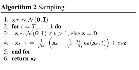
The first piece is a drift toward the clean image: it takes the current \(x_t\), asks \(\epsilon_\theta\) how much noise is in it, and subtracts that. This is exactly the reparameterized mean of Eq. (11), and because \(\epsilon_\theta\) is the score up to a scalar, it is one step of Langevin dynamics. The second piece, \(\sigma_t z\), is the kick: a fresh bit of Gaussian noise. Drift alone would collapse every sample onto a single point; kick alone would just keep adding noise. Together they are the Langevin balance, applied once per step.
(The code is this verbatim: p_sample (lines 186–198) is the drift-plus-kick line sample = model_mean + nonzero_mask * exp(0.5 * model_log_variance) * noise, with the drift folded into model_mean and the kick explicit; nonzero_mask is the “else \(z=0\)” branch. p_sample_loop (lines 200–219) is the \(t = T \to 1\) loop.)
noise levels schedule The score is only learnable at some noise levels. At large \(t\) the data has been smoothed almost to a Gaussian, so the score is nearly linear, easy to predict, and the sampler makes big, coarse moves. At small \(t\) the distribution is close to the real data, so the score is sharp, and the sampler makes fine, detail-level moves. Running the ladder from noisy to clean means no single step ever asks the network for more than a small, learnable piece.
That is annealed Langevin dynamics (Song & Ermon, 2019): start hot, cool gradually, use the score at each temperature.
(this video is the clearest explanation I have found of this whole thing)
7. What the bound buys
The three equations worth remembering
Forward closed form (Eq. 4) - start anywhere:
\[q(x_t\mid x_0) = \mathcal{N}(x_t; \sqrt{\bar{\alpha}_t}\,x_0, (1-\bar{\alpha}_t)I)\]Reverse parameterization (Eq. 11) - the network predicts noise, the mean is arithmetic:
\[\mu_\theta(x_t, t) = \frac{1}{\sqrt{\alpha_t}}\left(x_t - \frac{\beta_t}{\sqrt{1-\bar{\alpha}_t}}\,\epsilon_\theta(x_t, t)\right)\]Simplified objective (Eq. 14) - the loss is a noise MSE:
\[L_{\text{simple}} = \mathbb{E}_{t,x_0,\epsilon}\!\left[\left\|\epsilon - \epsilon_\theta\!\left(\sqrt{\bar{\alpha}_t}\,x_0 + \sqrt{1-\bar{\alpha}_t}\,\epsilon,\, t\right)\right\|^2\right]\]8. What this model is bad at, and what it is secretly doing
Limitations
- Likelihoods are not competitive: “our models do not have competitive log likelihoods compared to other likelihood-based models” (Section 1) - 3.75 bits/dim against 2.80 for Sparse Transformer.
- Sampling is slow: \(T = 1000\) sequential network evaluations per image (17 seconds per batch of 256 on a TPU v3-8; 300 seconds per batch of 128 at 256×256).
- Learned variances are unstable: “learning reverse process variances… leads to unstable training and poorer sample quality compared to fixed variances” (Section 4.2).
- The decoder is a heuristic, not a model. \(p_\theta(x_0\mid x_1)\) is a fixed bin-width discretization; the paper notes it “would be straightforward to instead incorporate a more powerful decoder like a conditional autoregressive model, but we leave that to future work.”
- Barely any hyperparameter search. The run is \(T=1000\), \(\beta_t\) linear \(10^{-4} \to 0.02\), batch size 128, EMA 0.9999, learning rate \(2\times10^{-4}\) - and of those, only the \(\beta_t\) schedule family was actually searched (constant/linear/quadratic, on CIFAR-10). \(T\), the batch size, the EMA decay, and the learning rate were all fixed without a sweep, and the learning rate had to be cut to \(2\times10^{-5}\) for the 256×256 models, which were unstable at the CIFAR-10 value. Dropout is the exception: swept over \(\{0.1,0.2,0.3,0.4\}\) on CIFAR-10, then set to zero elsewhere without a sweep.
Improved Denoising Diffusion Probabilistic Models addresses several of these directly - learned variance, a cosine schedule, a hybrid objective, importance sampling over \(t\), and strided sampling that cuts the step count by an order of magnitude.
9. The bottom line
DDPM’s contribution is less a new objective than a demonstration that a fairly old idea works at scale once three choices line up:
- The reverse process predicts noise \(\epsilon\) rather than the mean.
- Training uses the unweighted MSE on \(\epsilon\) - \(L_{\text{simple}}\), not the bound itself.
- The backbone is a U-Net with self-attention and group normalization.
Underneath, it is a variational bound on \(\log p_\theta(x_0)\) that decomposes into Gaussian KLs because the forward process was made fixed and therefore tractable. The \(\epsilon\)-parameterization connects that bound to denoising score matching and Langevin dynamics, and the simplified objective redirects capacity from easy denoising toward hard denoising.
Paper equation → code
| Math | Code | Line |
|---|---|---|
| §2.1 notation | __init__ |
64–81 |
| Eq. (4) forward closed form | q_sample |
101–111 |
| Eq. (7) posterior \(\tilde{\mu}_t,\tilde{\beta}_t\) | q_posterior_mean_variance |
113–126 |
| Eq. (8) the KL between the two means | normal_kl |
8–13 |
| Eq. (11) mean reparameterization | p_mean_variance |
128–168 |
| Eq. (14) \(L_{\text{simple}}\) | training_losses |
274–304 |
| Algorithm 2 sampler | p_sample / p_sample_loop |
186–219 |
| Eq. (5) the bound, in bits/dim | _vb_terms_bpd |
257–272 |
| progressive decoding | p_sample_loop_progressive |
221–253 |
| \(\beta\) schedule family | get_beta_schedule |
23–39 |
The defaults used for CIFAR-10 are eps / fixedlarge / mse, linear schedule \(10^{-4} \to 0.02\), \(T=1000\) (scripts/run_cifar.py, lines 130–137).
further reading
- Lilian Weng, What are Diffusion Models?
- Hugging Face, The Annotated Diffusion Model
- Yang Song, Generative Modeling by Estimating Gradients of the Data Distribution
breadcrumbs
part of the diffusion cluster, in reading order:
- diffusion-notes - the overview map of the whole family
- improved ddpm (2102.09672) - what ho et al leave on the table: learned variances, cosine schedule
- noise schedules, cfg & samplers (2305.08891) - the terminal-snr endgame of this schedule line
- kl divergence notes - the “gap = KL” step of the bound lives here too
todos
- re-derive the two forms of Eq. (3) once without peeking at the Jensen write-up - the bound’s spine.
- bridge to the continuous-time version (score SDE; the Yang Song post is already in further reading) - currently zero notes on that half.
- fold the ho-jonathanho code table into a runnable notebook check: reproduce one
_vb_terms_bpdnumber locally.