

The matrix calculus you need for deep learning
my notes on Parr & Howard, “The Matrix Calculus You Need For Deep Learning” (july 2018). their point: deep learning is mostly vector calculus - functions $f: \mathbb{R}^n \to \mathbb{R}$ reduced to one scalar (the loss) - so the single-variable intuition has to be upgraded: one equation at a time becomes a matrix of derivatives.
from scalar derivatives to the jacobian
start scalar: how does $xy$ change when we wiggle the variables? depends on which one - compute derivatives w.r.t. one parameter at a time, giving partial derivatives. for a single parameter, $\partial/\partial x$ and $d/dx$ coincide (for smooth enough functions); the paper prefers $d/dx$ to signal “scalar derivative”.
- gradients live in vector calculus: functions of $n$ scalar parameters → one scalar. the gradient stacks the partial derivatives.
- the Jacobian is the general object: for a function of $n$ variables producing $m$ outputs, with gradients as rows:
shape bookkeeping: the Jacobian is $m$ rows for $m$ equations, and $n$ wide if we differentiate w.r.t. $x$ (there are $n$ things to wiggle). the paper’s shape chart covers all four combinations of scalar/vector × scalar/vector inputs and outputs:
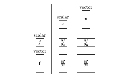
(careful when mixing sources: this paper puts gradients in rows; many ML texts stack gradients as columns. the transpose-flip is the #1 source of “my backprop shapes don’t match”.)
identity functions → the identity jacobian
take $f_i(x) = x_i$ (identity functions). applying the definition:
\[\frac{\partial F}{\partial x} = \begin{bmatrix} \frac{\partial x_1}{\partial x_1} & \frac{\partial x_1}{\partial x_2} & \cdots & \frac{\partial x_1}{\partial x_n}\\ \frac{\partial x_2}{\partial x_1} & \frac{\partial x_2}{\partial x_2} & \cdots & \frac{\partial x_2}{\partial x_n}\\ \cdots\\ \frac{\partial x_n}{\partial x_1} & \frac{\partial x_n}{\partial x_2} & \cdots & \frac{\partial x_n}{\partial x_n} \end{bmatrix} = \begin{bmatrix} 1 & 0 & \cdots & 0\\ 0 & 1 & \cdots & 0\\ \cdots\\ 0 & 0 & \cdots & 1 \end{bmatrix} = I\]the Jacobian of the identity function is the identity matrix.
elementwise operations → diagonal jacobians
any binary elementwise operation ($\bigcirc$ = Hadamard product, addition on matching indices, etc.) takes two vectors and returns one:
\[F(\vec{v}, \vec{w}) = \begin{bmatrix} f_1(\vec{v}) \bigcirc g_1(\vec{w})\\ f_2(\vec{v}) \bigcirc g_2(\vec{w})\\ \cdots\\ f_n(\vec{v}) \bigcirc g_n(\vec{w}) \end{bmatrix}\]take the Jacobian w.r.t. $v$: entry $(i,j)$ differentiates $f_i(v)\bigcirc g_i(w)$ w.r.t. $v_j$. because elements never interact across indices, everything off the diagonal is zero:
\[\frac{\partial F}{\partial v} = \begin{bmatrix} \frac{\partial f_1(\vec{v}) \bigcirc g_1(\vec{w})}{\partial v_1} & 0 & \cdots & 0\\ 0 & \frac{\partial f_2(\vec{v}) \bigcirc g_2(\vec{w})}{\partial v_2} & \cdots & 0\\ \cdots\\ 0 & 0 & \cdots & \frac{\partial f_n(\vec{v}) \bigcirc g_n(\vec{w})}{\partial v_n} \end{bmatrix} = \text{diag}\!\left(\frac{\partial f_1}{\partial v_1}, \frac{\partial f_2}{\partial v_2}, \dots, \frac{\partial f_n}{\partial v_n}\right)\]the Jacobian of every elementwise function is diagonal - “diagonal matrix”, not “diagonal vector” (a matrix with a diagonal, not a diagonal-shaped vector; the paper is clear on this). and the general element is $\frac{\partial f_i(v_i) \bigcirc g_i(w_i)}{\partial v_i}$.
worked example with numbers, since the paper’s own examples are symbolic: let $F = v \odot w$ with $v = \begin{bmatrix}2\3\end{bmatrix}$, $w = \begin{bmatrix}5\7\end{bmatrix}$. then $F = [10, 21]^\top$ and
\[\frac{\partial F}{\partial v} = \text{diag}(w) = \begin{bmatrix}5 & 0\\0 & 7\end{bmatrix}, \qquad \frac{\partial F}{\partial w} = \text{diag}(v) = \begin{bmatrix}2 & 0\\0 & 3\end{bmatrix}\]exactly what intuition says: wiggling $v_1$ by $\delta$ moves $F_1$ by $w_1\delta = 5\delta$ and leaves $F_2$ alone. diagonal. this is the reason elementwise nonlinearities (sigmoid, ReLU, tanh) never tangle gradients across coordinates in backprop - their Jacobians are diagonal, so they just scale the incoming gradient.
the vector chain rule
the total derivative of $f$ at a point = the best linear approximation of the function near that point, w.r.t. all arguments at once (with one variable, it collapses to the ordinary derivative). the total-derivative chain rule:
\[\frac{\partial f(u_1, u_2, \dots, u_{n+1})}{\partial x} = \sum_{i=1}^{n+1} \frac{\partial f}{\partial u_i}\frac{\partial u_i}{\partial x}\]the beauty of the vector version: it packages the total derivative automatically while keeping single-variable notational simplicity. state it as the theorem the images imply:
\[\frac{\partial f}{\partial x} = \frac{\partial f}{\partial g}\,\frac{\partial g}{\partial x} \qquad \text{(Jacobian } m \times k \text{ times } k \times n \text{ = } m \times n)\]where the middle variable $g$ has dimension $k$ ($m = \lvert f \rvert$, $n = \lvert x \rvert$, $k = \lvert g \rvert$):
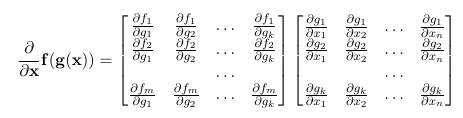
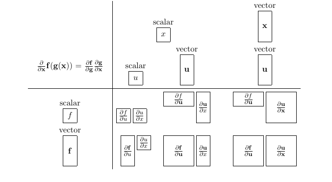
the Jacobian contains all combinations of $f_i$ w.r.t. $g_j$ and $g_i$ w.r.t. $x_j$; matrix multiplication then sums over the shared $k$ - which is exactly the total-derivative sum, but done for every output at once.
and the payoff direction: with “gradients are rows” + “elementwise ⇒ diagonal” + “chain rule ⇒ Jacobians multiply”, section 6 of the paper derives the differential of the neural-net cost w.r.t. weights and biases - the actual thing backprop computes. i deliberately never copied that derivation wholesale: read section 6 again and re-derive it on paper before writing it up.
papers
todos
- actually re-derive §6 (cost differential vs. $W$ and $b$), then write it up with a tiny 2-neuron numeric check.
- reconcile with the column-gradient convention other texts use (PyTorch docs, most textbooks) so i stop transposing shapes by hand.
- add the softmax-with-cross-entropy Jacobian shortcut (the paper covers it; classic interview trap).