


word2vec notes
the idea in one line: give every word a dense vector, chosen so that vectors of words appearing in similar contexts end up similar (the distributional hypothesis wearing math). mikolov et al’s papers are the source; my walkthrough leans on CS224n notes, Christophe Garon’s negative-sampling explainer, and Chris McCormick’s tutorials.
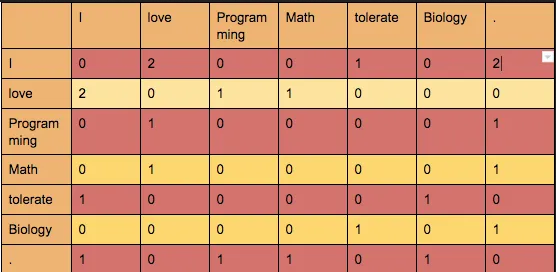
think about [[0.234, 0.4387, 0.46781]] as a position in a high-dimensional space: words with similar meaning sit close together, word groups cluster. and always ask: how is this data generated? word2vec generates its supervision by sliding over a corpus - no labels, just co-occurrence.
the setup
- big corpus of text; every word gets a vector.
- for each position $t$ there’s a center word $w_t$ and outside/context words $w_{t+j}$ within a window of size $m$.
- use the similarity of the vectors for center $c$ and context $o$ to compute the probability of $o$ given $c$.
- keep adjusting the vectors to maximize these probabilities.
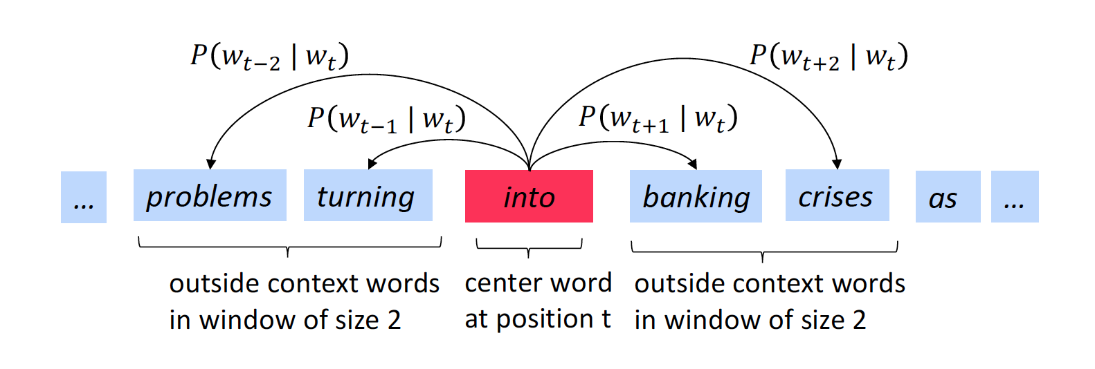
likelihood over the whole corpus (predicting every context word in the window around each center):
\[L(\theta) = \prod_{t=1}^{T}\prod_{-m \le j \le m,\ j \ne 0} P(w_{t+j} \mid w_t;\, \theta)\]we minimizing the negative log likelihood:
\[J(\theta) = -\frac{1}{T}\log L(\theta) = -\frac{1}{T}\sum_{t=1}^{T}\sum_{-m \le j \le m,\ j \ne 0} \log P(w_{t+j} \mid w_t;\, \theta)\]lower loss = better predictions everywhere on average.
two vectors per word
how do we actually compute $P(w_{t+j} \mid w_t)$? every word gets two vectors: $v_w$ used when the word is the center, $u_w$ used when it’s context. then a softmax over dot products:
\[P(o \mid c) = \frac{\exp(u_o^\top v_c)}{\sum_{w \in V} \exp(u_w^\top v_c)}\](the numerator is the observed context word’s vector dotted with the center - some write-ups leave it as U^T V_c with the observed word missing.)
- the dot product measures similarity: larger → more similar → higher probability of $o$ being near $c$.
- “soft”+”max”: see softmax notes.
this is the whole model. everything else is making $\sum_{w \in V}$ survivable.
the practical picture (skip-gram)
you can’t feed text strings to a network, so: build a vocabulary (say 10,000 words), represent “ants” as a one-hot vector of 10,000 components. the model is a two-layer network:
- hidden layer: a $10000 \times 300$ weight matrix - 300 features per word. multiply the one-hot by it and you effectively just select one row:
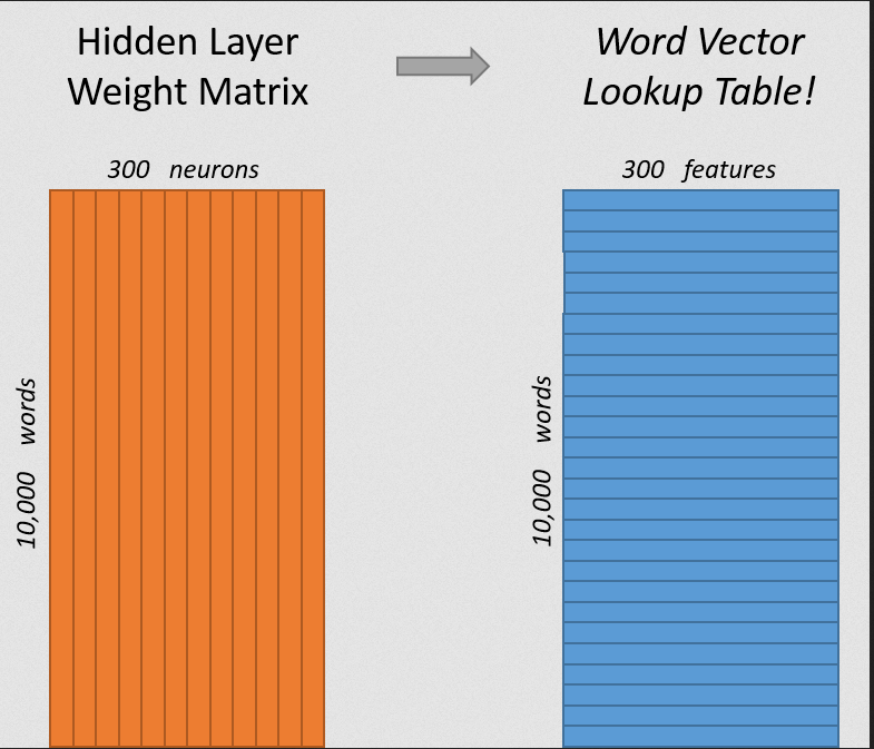
the hidden layer is a lookup table; its output is the word vector for the input word. (this is also why the gradient never touches the other 9,999 rows of that row’s step - the update cost per sample is tiny.)
- output layer: softmax regression over the vocabulary, producing the probability that each word in the corpus is a nearby word.
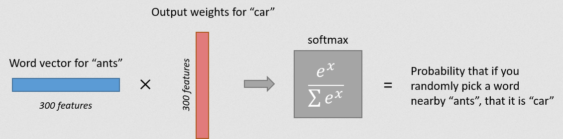
the objective, concretely: minimize the average log-probability of the true context words around the input.
a word vector is never “predicted” - context probabilities are predicted. the vectors are learned inputs, refined only to drive down the prediction loss; the word’s “meaning” ends up embedded in those weights. (that framing - vectors as learned representation, not output - cleaned up a misconception i carried for a while.)
cbow vs skip-gram
- CBOW: predict the focus word from the averaged context (“an efficient method for … vector” → “learning”). faster, better representations for frequent words.
- Skip-gram: predict each context word from the focus word (“learning” → all 8 context words). slower, better for rare words - each rare occurrence becomes multiple training signals.
the denominator problem, solved twice
the softmax denominator normalizes over the entire vocabulary - hundreds of thousands to millions of terms per training sample. that’s the wall. two ways around it:
hierarchical softmax
represent the vocabulary as a binary tree with words as leaves; the probability of a word is the probability of a random walk from root to its leaf (“define this probability as the probability of a random walk starting from the root ending at the leaf in question”). cost drops from $O(V)$ to $O(\log V)$ per sample.
negative sampling (the one everyone uses)
reformulate: forget predicting the whole distribution. for each true (center, context) pair, draw $k$ words not in the context and train on a binary discrimination:
\[\log \sigma(u_o^\top v_c) + \sum_{j=1}^{k} \mathbb{E}_{w_j \sim P_n(w)} \big[\log \sigma(-u_{w_j}^\top v_c)\big]\](this is the paper’s form; transcription variants floating around tend to lose the indices.)
terms: the first pushes the real context word’s similarity up; the $k$ expectation terms push randomly-drawn words’ similarity down. update cost per sample: the positive output unit + $k$ negative units. with $k = 5$: 6 output neurons out of 10,000 → ~1,800 of 3M weights touched → 0.06% of the output layer per sample.
- $k$: 5-20 for small datasets, 2-5 for large ones (paper’s guidance).
- $P_n(w)$: the noise distribution, the unigram frequency raised to $\frac{3}{4}$:
frequent words are more likely negatives (“the”, “of” need pushing away from everything), but the $\frac{3}{4}$ exponent tames them relative to raw frequency - a dampener found empirically, not derived. (why 3/4? the paper’s answer is basically “it worked better” - see todos.)
- implementation trivia worth keeping: the C code builds a 100M-element unigram table where word $i$’s index appears $P(w_i) \cdot 10^8$ times; sampling a negative = one random integer + an array lookup. no aliasing math, just memory for speed.
subsampling frequent words
“the”, “in”, “a” carry little information but dominate counts, skewing training toward them. mikolov’s subsampling: discard word $w_i$ with probability
\[P(\text{discard } w_i) = 1 - \sqrt{\frac{t}{f(w_i)}}\]with $t$ a threshold, typically $\sim 10^{-5}$. (watch the $t$: without it - $1 - \sqrt{1/f(w)}$ - the discard probability is unbounded by any cap, and $t$ is exactly the cap it wants. load-bearing.) frequent words get randomly dropped, keeping the training set balanced and implicitly widening the effective context windows.
analogies: the result everyone knows
the paper this note is really about is the vector-arithmetic one: king − man + woman ≈ queen. the offsets between word pairs encode relations (“gender”, “tense”…) that survive addition - that’s vector-oriented reasoning, and it’s what made embeddings culturally famous. run it: subtract, add, then cosine-search the vocabulary for the nearest non-input word.
applied word2vec (worth skimming once)
- music recommendations (Anghami, via a TDS write-up - link rotted by now) - playlists as sentences.
- Airbnb listing embeddings - bookings as context; embeddings for search ranking.
- Yahoo Mail ads - user purchase/interaction sequences as sentences; then the trick: don’t recommend from the same cluster the purchased item sits in - find which clusters users move to next, recommend the top-$k$ items from those clusters instead (20 products/day).
papers
- efficient estimation of word representations (CBOW + skip-gram): https://arxiv.org/abs/1301.3781
- distributed representations of words and phrases (negative sampling, subsampling, phrases): https://arxiv.org/abs/1310.4546
- vector-oriented reasoning (king−man+woman=queen): https://aclanthology.org/N13-1090
- applied: yahoo mail ads https://arxiv.org/abs/1607.01869, yahoo e-comm in inbox https://arxiv.org/abs/1606.07154
todos
- the gradient/update rules i keep skipping (CS224n derives them): $\partial J/\partial v_c = U(\hat{y} - y)$, $\partial J/\partial u_o = v_c(\hat{y}_o - y_o)$ - write the derivation as its own section.
- hierarchical softmax: path probability $p(w) = \prod_{i=1}^{L(w)} \sigma(\pm b_i^\top v)$ with the path-code signs written out.
- gloVe vs fastText - counting-based (co-occurrence matrix factorization) vs char-ngram-based; one paragraph each, so this note covers the whole embedding menu.
- why exactly $\frac{3}{4}$ in the noise distribution - chase down whether anyone has a better justification than “empirically”.