

FCN notes
Long, Shelhamer, Darrell 2015 (+ the 2016 journal version): the paper that turned classification nets into segmentation machines. pairs naturally with my U-Net notes - U-Net is the idea taken one refinement further.
why not just a classifier?
semantic segmentation is not image classification: the goal is a dense prediction - a class for every pixel - not one label for the image. so the final fully-connected layers (the “classifier head”) are useless here and get dropped: what we want is the feature extraction machinery, plus something to separate the image into segments with.
the catch: convnets shrink the image as it flows through, mostly via max-pooling (and strided convs). by the end of a classification backbone the “map” is coarse - a $\tfrac{1}{32}$-ish scale sketch. so segmentation needs to get resolution back. that’s the whole problem FCN solves: upsample in-network, and do it learnable.
from classifier to dense fcn
the conversion recipe, from the paper:
- decapitate: drop the final classifier layer.
- convolutionalize: view every fully connected layer as a convolution with kernels covering its whole input region. (an FC layer with fixed input size is just a $1\times1$ conv over a flattened map - recasting it makes the net accept arbitrary input sizes and emit classification maps.)
- score: append a $1\times1$ convolution with 21 channels (PASCAL classes + background) - now every coarse output location carries per-class scores.
- upsample: a (backward) convolution layer bilinearly upsamples the coarse scores to pixelwise output.
each convnet layer is just a 3-D array $h \times w \times d$, and “receptive field” is the concept to keep: a location in a deeper layer corresponds to the patch of image pixels it’s path-connected to.

training details worth keeping (the $10^{-3}$/$10^{-4}$/$5\times10^{-5}$ learning rates for FCN-AlexNet/VGG16/GoogLeNet - the paper’s PDF text layer mangles the last one into $5^{-5}$, and the weight decay $5\times10^{-4}$ or $2\times10^{-4}$ gets the same treatment): SGD with momentum 0.9, gradients accumulated over 20 images, doubled lr for biases, class scoring layer zero-initialized (random init gave nothing), dropout where the original net had it.
upsampling = transposed convolution
bilinear interpolation computes each output from the nearest four inputs by a position-dependent linear map - fine, but fixed. the reframing that unlocks learning: upsampling with factor $f$ = convolution with a fractional input stride $1/f$, so as long as $f$ is integral you can implement it as a transposed convolution with output stride $f$.
the honest mental model (the “filters slide over the input instead” folklore is the confusing version): a transposed conv is the ordinary convolution whose backward pass is the operation you want - the forward of transposed-conv is the backward of conv. trivially implemented by swapping the stride/padding roles, and - the key point - not required to stay bilinear: the filter is learnable, in-network, trained by backprop from the pixelwise loss. a stack of deconv layers + activations can even learn non-linear upsampling.
a conflation worth flagging, since summaries repeat it: zero-padding does not upsample (“padding maintains spatial dimensions”) - no: padding preserves/controls size during convolution; the resolution increase comes from the transposed stride. two separate knobs.
skip architectures - the actual trick
here’s the limitation: the stride of the final prediction limits how much detail survives upsampling. too much spatial information died in all that downsampling.
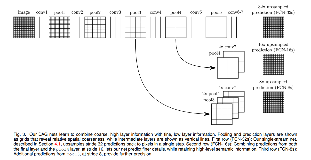
the fix: add skips that fuse shallower layers with finer strides into the prediction. this turns the line topology into a DAG: shallower layers have smaller receptive fields and see fewer pixels, so they make locally precise predictions; deep layers make globally consistent ones. fuse them and local predictions start respecting global structure.
mechanics of a skip, as the paper does it:
- align: layers to fuse must match in scale - upsample the lower-res one in-network, then crop away the padding fringe so dimensions correspond exactly.
- fuse cheaply: concatenation followed by a $1\times1$ “score layer”. since both are linear, they commute the concat into a sum of per-layer scores - no giant concatenated tensor in memory.
- zero-init the score layer when a skip is added so it doesn’t disturb the streams already learning.
- (max fusion was tried and dropped - gradient switching makes learning flaky.)
naming conventions: FCN-16s = VGG16 backbone + skip from pool4 (stride 16), FCN-8s adds the pool3 skip (stride 8). each skip halves the effective stride. the interpolation layers initialize to bilinear but stay learnable.
vgg16, concretely
walkthrough for the standard recipe: take VGG16 up through pool5 and its FC stack ($1{\times}1{\times}4096 \to 1{\times}1{\times}4096 \to 1000$); replace the three FC layers with $1\times1$ convs (to 21 classes), then a deconvolution for upsampling; wire the pool4/pool3 skips as above. (my source walkthrough: Mohit Gaikwad’s post; skip-connection details are §4.2 of the paper.)
fine-tuning and the background-model experiment
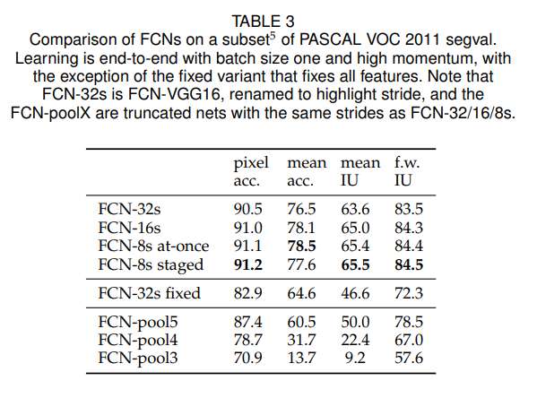
- fine-tuning all layers through the whole net is what matters: fine-tuning only the output classifier gets you 73% of full performance. staged fine-tuning: 36 h on one GPU; FCN-8s trained all-at-once reaches comparable accuracy in half the time; training from scratch lands way lower - transfer the representation.
- the null-background experiment: replace the learned background class with a constant-zero score (sigmoid cross-entropy instead of softmax so classes compete less), and the net scores only 1 point below the reference - while saving <0.1% of parameters. conclusion: a dedicated background model is nice, not vital. i like this experiment; it’s the kind of “is this assumption load-bearing?” ablation more papers should run.
papers & sources
- FCN: https://arxiv.org/abs/1411.4038 (journal ver: https://arxiv.org/abs/1605.06211)
todos
- add the actual PASCAL VOC mIoU numbers (FCN-32s vs 16s vs 8s vs prior SOTA) - these notes kept method text but no results table.
- transposed conv arithmetic (output size formula from kernel/stride/padding) deserves its own worked example - my earlier padding confusion started there.