

U-Net notes
Ronneberger, Fischer, Brox 2015: the encoder-decoder with dense skip connections that became the default biomedical segmentation backbone (and the skeleton under SegMamba’s modern descendants). read alongside my FCN notes - U-Net is FCN’s skip idea, tightened.
fcn vs u-net, stated carefully
the folk summary (“FCN upsamples the final features; U-Net adds shortcuts”) undersells both sides. FCN-8s already fuses shallow layers (pool3, pool4) into its prediction. the honest distinction: FCN fuses by scoring each stream with $1\times1$ convs and summing the scores at the end; U-Net instead concatenates full encoder feature maps into every decoder level, so the shallow detail is available at every upsampling step, not just fused into the final score. denser reuse, stronger multi-scale mixing - and the decoder does more of the work.
architecture
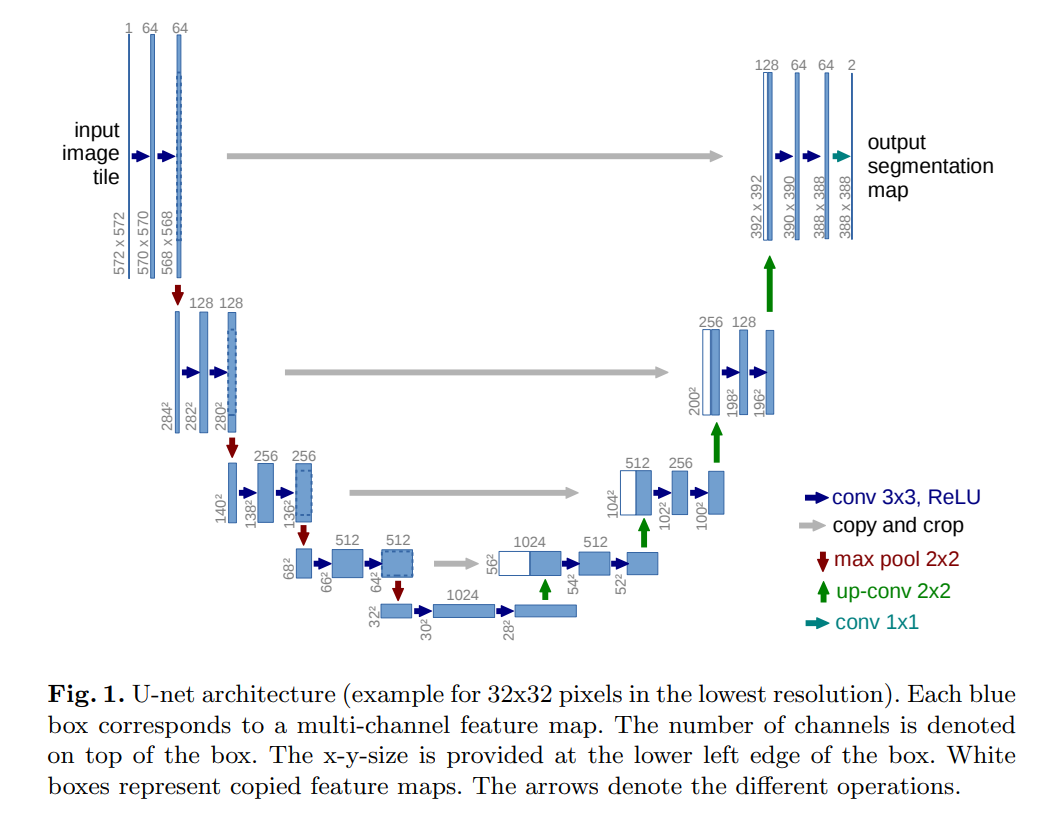
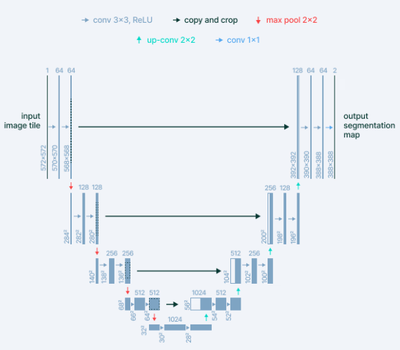
- contracting path (encoder): repeated blocks of two $3\times3$ convolutions (unpadded - border pixels die at every conv) + ReLU, then $2\times2$ max-pool (stride 2) for downsampling. channels double at every pooling step.
- expansive path (decoder): every step is an upsampling (feature map upsampled) followed by a $2\times2$ transposed convolution (“up-conv”) that halves the channels, then concatenation with the correspondingly cropped encoder feature map, then two $3\times3$ convs + ReLU.
- final $1\times1$ conv maps the 64-component feature vector to the class count.
total: 23 convolutional layers - and the correct split (the “11 encoder / 11 decoder” you’ll meet in summaries doesn’t survive contact with the architecture): 10 in the encoder (5 blocks × 2 convs), 12 in the decoder (4 upsampling steps × (1 up-conv + 2 convs)), plus the final $1\times1$.
the cropping on skips exists because of those unpadded convs: the encoder maps have lost border pixels, so the decoder map doesn’t line up without trimming.
training
- plain SGD (Caffe), momentum 0.99 and batch size 1: unpadded convs mean the output is smaller than the input, so the authors favor big input tiles over big batches and let a huge momentum pool many previously-seen samples into each update.
- overlap-tile strategy: to segment images larger than GPU memory, run the network on tiles with the surrounding context visible, so every interior prediction sees enough border context - and choose tile shapes that keep every $2\times2$ pooling on even x/y sizes for seamless tiling of the output.
- loss: pixel-wise softmax over the final feature map + cross entropy. reframed: turn segmentation into per-pixel multiclass classification - every pixel must land in some class. performed very well against the traditional alternatives.
- weight map to fix class imbalance and make the network learn the thin borders between touching cells:
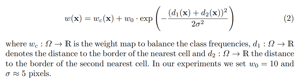
in words: each pixel carries a weight combining a class-frequency balancing term $w_c(x)$ with a border term that boosts pixels near separations between touching cells, falling off with distance $d_1(x) + d_2(x)$ to the nearest cell borders. the separation border itself is computed with morphological operations. this is what lets the model segment cells individually - the loss literally shapes the space between them.
- initialization: alternating conv/ReLU needs unit-variance activations out of the gate, so weights come from $\mathcal{N}(0, \sqrt{2/N})$ with $N$ = incoming nodes ($3\times3$ conv × 64 channels → $N = 9 \cdot 64 = 576$). the paper PDF’s “std of p 2/N” is a radical-garble of $\sqrt{2/N}$ - the He-style init.
one quirk to sit with: the paper never justifies the unpadded design beyond the border-crop story, but the modern default is padded convs + same-size outputs, precisely to avoid the 92-pixels-lost-per-side dance. the usually-quoted reason (“didn’t want to introduce segmentation errors at the margin”) is only half the story - the other half is that with unpadded convs, overlap-tile inference requires context margin anyway, so the border loss is by design, not an accident. for a $572 \times 572$ input the output is $388 \times 388$ (~68% linear scale, 92 px gone per side).
what later practice changed
- dice loss vs cross-entropy for the extreme class imbalance of biomedical masks - robust where CE gets dominated by background:

- the original elastic deformation augmentation (random elastic warps of the images) was the paper’s headline data trick for learning deformation invariance cheaply - worth a line in every U-Net retelling, and skipped as often as not (the SegMamba recipe still uses it, 9 years later).
- pixel shuffle as an alternative upsampler (borrowed from super-resolution nets like SRGAN): conv from $C \times H \times W$ to $(Cr^2) \times H \times W$, then reshape pixel-wise (“mosaic fashion”) to $C \times Hr \times Wr$ - learned upsampling without transposed convs.
- reference implementation: Pytorch-UNet.
papers & sources
- U-Net: https://arxiv.org/abs/1505.04597
- walkthroughs used above: TDS understanding U-Net, TDS U-Net, datature blog
todos
- the weight-map formula: the screenshot above carries the equation; i still owe the text version with the $w_c$, $w_0$, $\sigma$ roles spelled out and a worked example.
- run the numbers on unpadded U-Net once (which conv eats how many border pixels; why exactly 92 px/side at 572→388) and annotate the architecture figure.
- dice loss: derive the formula from the set-overlap definition and note where it’s numerically unstable (denominator at empty prediction) - these notes keep only the intuition.