

Kalman filter notes
start with the problem: estimate the state of a random process from measurements that are noisy. the measurement is the effect, the state is the cause:
\[m = \beta \, s + \epsilon\]a simple linear relation, with $\epsilon$ as noise. if state estimation is good, you can keep measuring even when the signal is bad. inferring unobserved variables from observed ones - statistics calls that a latent variable problem.
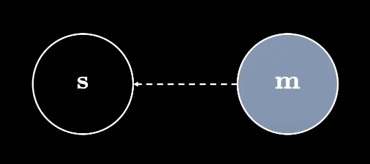
so: $s$ is unknown, and given the effect $m$ we want the cause. bayes rule does exactly this:
\[p_\theta(s \mid m) = \frac{p_\theta(m \mid s)\, p_\theta(s)}{p_\theta(m)}\]- $p(s)$ - belief about the state without any data → prior
- $p(m \mid s)$ - probability of the measurement given the state → likelihood
- $p(s \mid m)$ - prior updated by the measurements → posterior
- $p(m)$ - evidence, just a normalizing constant making it a valid distribution
the running theme: start with a belief about the state, update the belief as measurements arrive.
making it a sequence
now connect it to my SSM notes: assume the states form a first-order markov chain, and the measurements are independent of each other given the states (if you can model state-to-state transitions, modeling measurement-to-measurement transitions is redundant). throw in a picture:
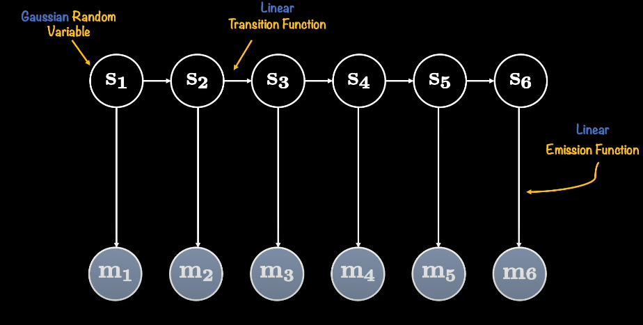
this kind of model is a linear-Gaussian state space model - the states live in gaussian space. and be precise about why gaussian here: not to shrink the normalizer ($p(m)$ is a constant either way), but because the gaussian is its own conjugate prior - the posterior after a linear-Gaussian update stays Gaussian, so the whole filter remains closed-form instead of turning into integration over an arbitrary distribution.
- linear transition function: $s_k = A_{k-1} s_{k-1} + q_{k-1}$ - $A$ transition matrix, $q$ process noise
- linear emission function: $m_k = H_k s_k + r_k$ - $H$ emission matrix, $r$ measurement noise (index-slip trap: $H$ acts on the current state $s_k$; $A$ is the one that trails with $k-1$ conventions)
the ssm dictionary maps straight across:
| kalman/lg-ssm | discrete SSM |
|---|---|
| hidden state $s_k$ | $h_k$ |
| transition $s_k = A_{k-1}s_{k-1} + q_{k-1}$ | state eq. $h’(t) = Ah(t) + Bx(t)$ |
| emission $m_k = H_k s_k + r_k$ | output eq. $y(t) = Ch(t)$ |
inference mode
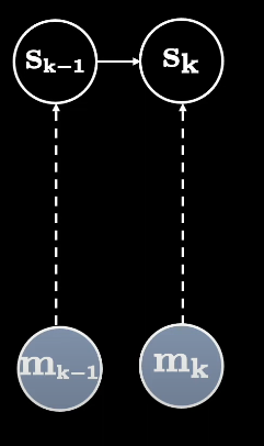
goal: the belief about the state at any step $k$, given all measurements so far. the recursive loop is:
- we hold a posterior over $s_{k-1}$ given $m_{k-1}$
- we want $p(s_k \mid m_{k-1})$, but there’s no direct path from $m_{k-1}$ to $s_k$ - we go through the transition. that marginalization is the Chapman-Kolmogorov equation (a “trick for now, intuition later” in my own notes - see todos)
bayesian filtering = predict + update
1. predict step (Chapman-Kolmogorov marginalization over the previous state):
\[p(s_k \mid m_{k-1}) = \int p(s_k \mid s_{k-1})\, p(s_{k-1} \mid m_{k-1})\, ds_{k-1}\]2. update step (bayes rule on the new measurement):
\[p(s_k \mid m_k) = \frac{p(m_k \mid s_k)\, p(s_k \mid m_{k-1})}{\mathcal{N}_k}\]and that’s the entire skeleton of every bayesian filter: predict, update, repeat. the linear-Gaussian SSM here is literally the ancestor of the whole h' = Ah + Bx lineage in my ssm notes.
papers & sources
- kalman 1960: https://courses.cs.duke.edu/compsci527/cps274/fall11/papers/Kalman60.pdf
- modern derivation walk: https://arxiv.org/pdf/1910.03558
- lecture that got me started: https://www.youtube.com/watch?v=-DiZGpAh7T4
todos
- the part the note is named after is still missing: the kalman gain $K$, the covariance predict/update pair, and explicit $Q$, $R$ noise covariances. everything above is the wrapper; the filter itself is the next sitting.
- chapman-kolmogorov: get the intuition, not just the integral trick (it’s “total probability along the chain” - write it up when done).
- connect $H$ here to the observation matrix in my SSM notes $C$, and note where the neural versions diverge (no noise covariances, learned $A$).