

SSM notes
i kept hearing “SSMs are just RNNs with better press” so i sat down and worked the lineage from the top: transformers and their cost problem, the plain-vanilla state space model, what discretization really does, and the convolution view that makes the whole thing trainable. most of the walkthrough below leans on Maarten Grootendorst’s visual guide, The Gradient’s Mamba explained, and Sasha Rush’s annotated S4, with control-theory stuff from tinkerd and libretexts sprinkled in. the deeper parts live in their own notes: HiPPO, S4, Mamba.
the tradeoff that starts everything
transformers are extremely effective, and extremely not efficient. every token can look back at every earlier token, which means caching detailed information about each one in the KV cache. that pairwise communication makes a training forward pass $O(n^2)$ and each autoregressive step $O(n)$ - as context grows the model gets slower. the KV cache is also $O(n)$ space, so the dreaded CUDA OOM shows up right on schedule. and you can’t just buy your way out: latency grows quadratically, so more GPUs don’t fix the slowness.
plain RNNs are the exact opposite tradeoff. they forget almost everything, keeping a small summary in the hidden state and discarding the rest. discarded information can’t be recovered, so they’re less effective - but the state is small, so they’re as efficient as it gets.
a state space model (SSM) is the attempt to have it both ways: RNN-like efficiency, more transformer-like memory.
what a state space model actually is
an SSM is a control-systems description of any system that takes inputs, maintains an internal state, and produces outputs - where the output depends on both the input and the state, and the state itself evolves as inputs arrive.
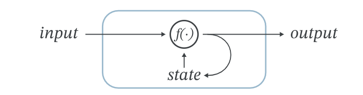
at time $t$, an SSM
- maps an input sequence $x(t)$
- to a latent state $h(t)$
- and derives an output $y(t)$
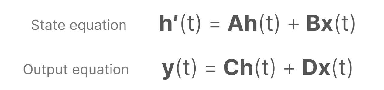
with the state evolving continuously per this equation:
\(h'(t) = Ah(t) + Bx(t)\) \(y(t) = Ch(t) + Dx(t)\)
the four matrices have clean jobs:
| matrix | name | job |
|---|---|---|
| $A$ | state transition | how the state evolves - “how should i forget the less relevant parts of the state over time?” |
| $B$ | input matrix | what part of the new input makes it into the state |
| $C$ | output matrix | how to read a prediction out of the state |
| $D$ | feedthrough | how the raw input skips straight into the output - basically a skip connection |
the maze framing made it click for me: $x(t)$ is “the screen moved left and down”, $h(t)$ is the state (“distance to the exit, x/y position”), $y(t)$ is the action (“move left again”). one thing to note: unlike an RNN it takes a continuous function-to-function view, not a discrete sequence-to-sequence view - we’ll fix that in the discretization section.
the temple-run intuition for why a small state can still be super useful: the state changes by known dynamics, so a small new observation is enough to nudge a mostly-predictable state. the top of the screen doesn’t just scroll, its velocity tells you the game is speeding up, so limited observations still pin down the overall dynamics pretty fast. most of the screen isn’t new - it’s a continuation of the previous state’s natural motion.
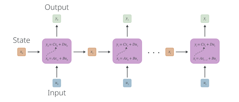
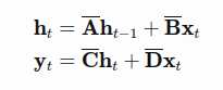
at each discrete step $t$ the hidden state $h_t$ carries information about all inputs up to and including $x_t$. one extra parameter $\Delta$ controls the interval between steps - it’ll matter a lot in a bit.
discretization - from functions to sequences
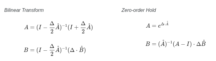
real data (text) is discrete, but the model above is continuous, so we discretize. this is a well-studied problem in control theory; SSM papers use the bilinear transform and zero-order hold, and the Euler method shows up as the naive baseline.
- Euler: the dumb one. $\bar{A} = I + \Delta A$, $\bar{B} = \Delta B$. it treats the rate of change as constant over the step, so the approximation drifts off the real curve the longer you go.


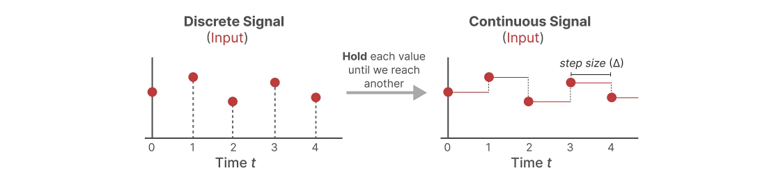
- Zero-order hold (ZOH): before running the continuous model, hold the current discrete value constant until the next one arrives. that synthesizes a continuous signal the SSM can actually consume, with $\Delta$ as the hold interval (the resolution of the input). the discrete update comes out as $\bar{A} = e^{\Delta A}$, $\bar{B} = A^{-1}(e^{\Delta A} - I)B$.

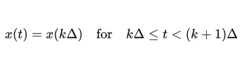
- Bilinear (trapezoid): averages the endpoint dynamics instead of pinning one - $\bar{A} = (I - \tfrac{\Delta}{2}A)^{-1}(I + \tfrac{\Delta}{2}A)$, $\bar{B} = (I - \tfrac{\Delta}{2}A)^{-1}\Delta B$.
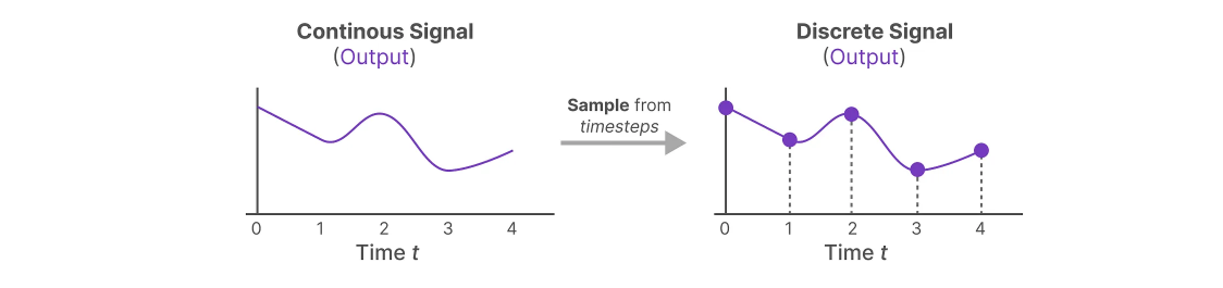
after discretization we go from function-to-function $x(t) \to y(t)$ to an honest sequence-to-sequence $x_k \to y_k$, with discretized parameters $\bar{A}, \bar{B}$ derived from the learned step size $\Delta$ and fixed choices of transform. $\Delta$ is the sampling interval - the exponential of $A$ scaled by $\Delta$ captures state evolution across the gap, and $\bar{B}$ is derived so the input’s influence over the interval stays consistent with the continuous dynamics.
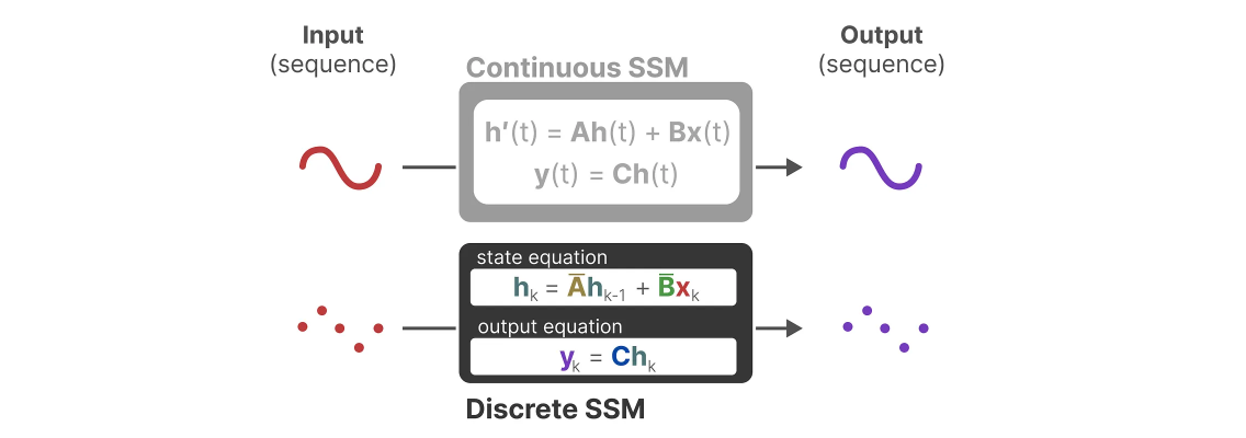
fine print that confused me the first time (the annotated S4 is the source):
- papers drop $\bar{D}$ from the exposition because it “can be viewed as a skip connection that does not interact with the state” - but the real S4 and Mamba implementations both still parameterize it. i agree with annotated S4: keep it in the math, it costs one term.
- $C$ isn’t really discretized at all: in Mamba there’s no $\bar{C}$, and in S4 the “discretization” of $C$ is just the identity. don’t let this bother you.
- three methods exist, euler is the weakest of them, but the real choice is nuanced between ZOH and bilinear. the S4 paper uses bilinear, Mamba highlights ZOH. (my earlier notes said “ZOH gives a better approximation hence that’s used in the paper” - no. that’s wrong; check which paper you’re standing in before repeating it.)
- one musing: the discretization functions are fixed and only the step size is learned. that goes against my own DL instinct of “let the model learn everything” - how far could learned discretization functions go instead? unexplored as far as i can tell.
if you’ve ever looked at an RNN this should feel extremely familiar:
\(h_k = \bar{A}h_{k-1} + \bar{B}x_k\) \(y_k = Ch_k + Dx_k\)
some input $x$ gets combined with the previous hidden state by a transform to make the new hidden state, and the hidden state makes the output. trust your instincts, it’s an RNN.
the convolution view
here’s the part that makes SSMs more than RNNs. unroll the recurrence with $h_{-1} = 0$:
\(h_0 = \bar{B}x_0\) \(h_1 = \bar{A}\bar{B}x_0 + \bar{B}x_1\) \(h_2 = \bar{A}^2\bar{B}x_0 + \bar{A}\bar{B}x_1 + \bar{B}x_2\) \(h_t = \sum_{j=0}^{t} \bar{A}^{t-j} \bar{B}\, x_j\)
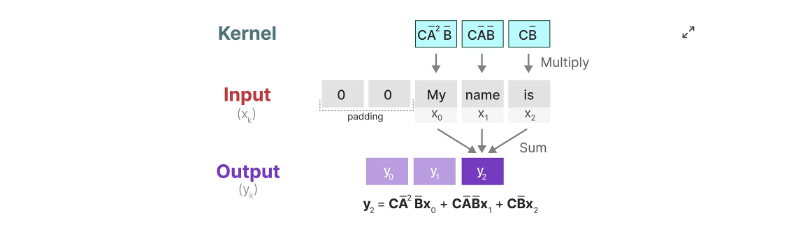
every term is $\bar{A}^{k}\bar{B}$ applied to a shifted input - so the whole state is a convolution of the input with a fixed kernel. fold $C$ in and write the output directly:
\[y_t = C(\bar{K} * x)_t + Dx_t \qquad \bar{K} = (C\bar{B},\; C\bar{A}\bar{B},\; C\bar{A}^2\bar{B},\; \dots)\]so one layer has two hats:
- recurrent: $h_k = \bar{A}h_{k-1} + \bar{B}x_k$ - $O(1)$ per step, constant memory, right for inference.
- convolutional: $y = \bar{K} * x$ - every position in parallel, right for training.
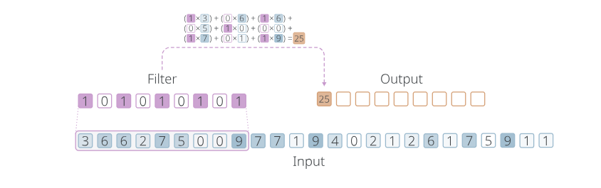
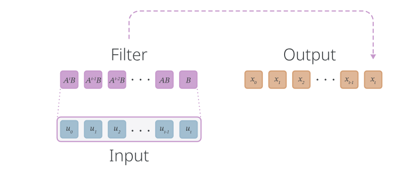
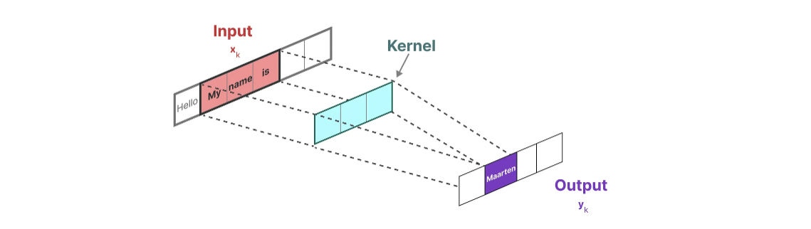
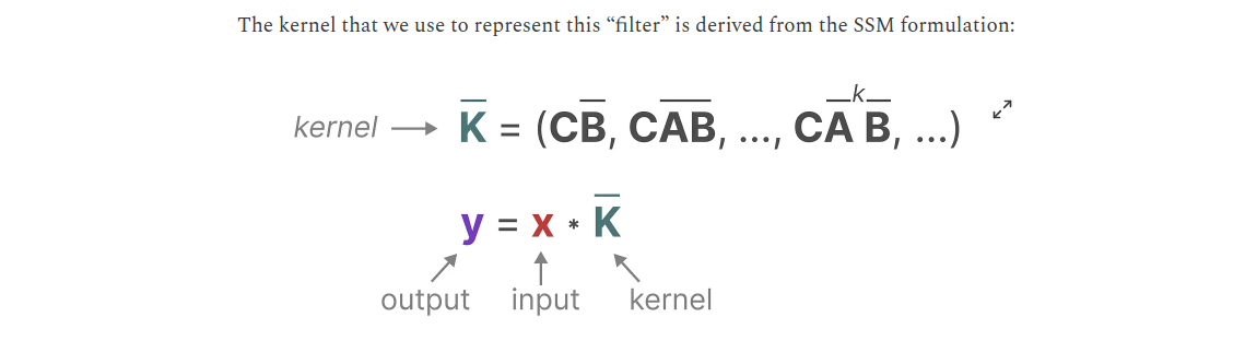
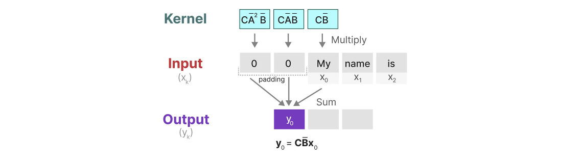
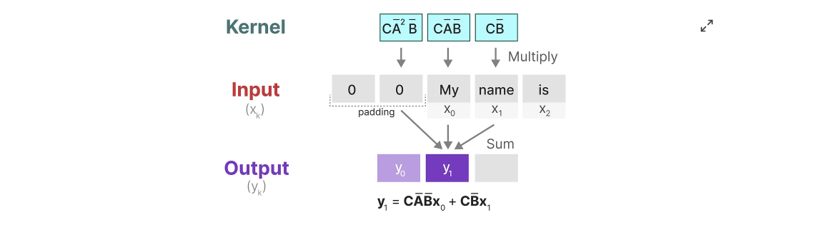
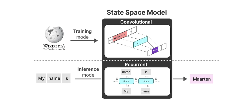
train conv, infer recurrent. (the kernel is fixed across inputs though - which is exactly the next problem.)
linear time invariance - the ceiling
everything above shares one property: LTI, linear time invariance. $\bar{A}$, $\bar{B}$, $\bar{C}$ are the same for every timestep. the model treats the first token and the ten-thousandth token with identical machinery, regardless of what’s in them. a static representation that isn’t content-aware.
no bueno. Mamba fixes this, and everything in between is this lineage:
- HiPPO - the structure of $A$ is what decides which parts of the previous state survive. HiPPO is the recipe for that structure: a principled way to compress the entire input history into the state. the structure of $A$ becomes the memory of the model itself.
- LSSL - one layer, three interchangeable views (recurrent / conv / continuous-time), and the realization that naive $A$ is impossible to learn without structure.
- S4 - LTI + structured (HiPPO) + diagonalized $A$ with clever kernels.
- H3 - SSM machinery wired specifically to do associative recall.
- Mamba - make $B$, $C$ and $\Delta$ input-dependent. selectivity. no more LTI.
- MLLA - and then you realize Mamba was linear attention wearing a control-theory costume.
papers i’m chipping through
- HiPPO: https://arxiv.org/pdf/2008.07669
- LSSL: https://arxiv.org/abs/2110.13985
- S4: https://arxiv.org/abs/2111.00396
- SaShiMi (S4 for raw audio - Hurwitz stability fix): https://arxiv.org/abs/2202.09729
- DSS (diagonal state spaces, no low-rank needed): https://arxiv.org/abs/2203.14343
- S4D: https://arxiv.org/abs/2206.11893
- H3: https://arxiv.org/abs/2212.14052
- LRU (“resurrecting rnns” - it studies SSMs and where the theory actually fails): https://arxiv.org/abs/2303.06349
- Mamba: https://arxiv.org/abs/2312.00752
useful videos: state space coordinates, discrete control playlist, mamba deep dive, mamba intuition, selective SSM breakdown
todos
- connect this linear-Gaussian SSM to my Kalman filter notes properly: predict = Chapman-Kolmogorov, update = Bayes, and neither note closes the loop yet - this whole lineage literally descends from the filter.
- study ODEs + Laplace transform (the control playlist above) before re-deriving the HiPPO ODE - right now i’m trusting the result instead of the derivation.
- the “plug-in state cartridges” idea from The Gradient: train a state once (pure compression, no gradients) and load it at inference for zero-compute in-context learning. worth chasing: has anyone actually built this?
- learned discretization functions (not just learned $\Delta$) - does anyone have a paper on this?
- revisit the LSSL “convolutions forward” gap the early draft never filled - covered by the kernel math above now, but walk it again inside the S4 note.