

Mamba notes
Mamba is the point in the SSM lineage where the model stops treating every token the same way. this note covers the selectivity idea, a minimal PyTorch implementation, and the hardware-aware algorithm that keeps it fast. the SSM/discretization basics are in SSM notes and the initialization story in S4 notes - not re-explained here. main sources: Mamba paper, The Gradient’s Mamba explained, James Chen’s walkthrough, and two videos: one, the really detailed one, referenced by the authors.
from time-invariant to time-variant
the SSM update from my SSM notes, using the discretized parameters (that note’s shorthand drops the bars - below, $A(t), B(t)$ mean the discretized operators for step $t$):
\[h_t = A h_{t-1} + B x_t \qquad y_t = C h_t + D x_t \qquad \text{(time-invariant: same } A,B,C,D \text{ every step)}\] \[h_t = A(t) h_{t-1} + B(t) x_t \qquad y_t = C(t) h_t + D(t) x_t \qquad \text{(time-variant)}\]Mamba is time-variant on $B$, $C$ and the step size $\Delta$: they’re computed at each timestep from the current input. we don’t learn the parameters directly - we learn the parameters of linear projections $s_B(x), s_C(x), s_\Delta(x)$ that produce them from the input $x$.
the mamba block
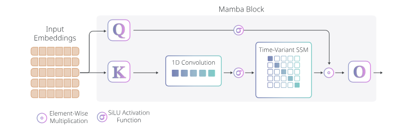
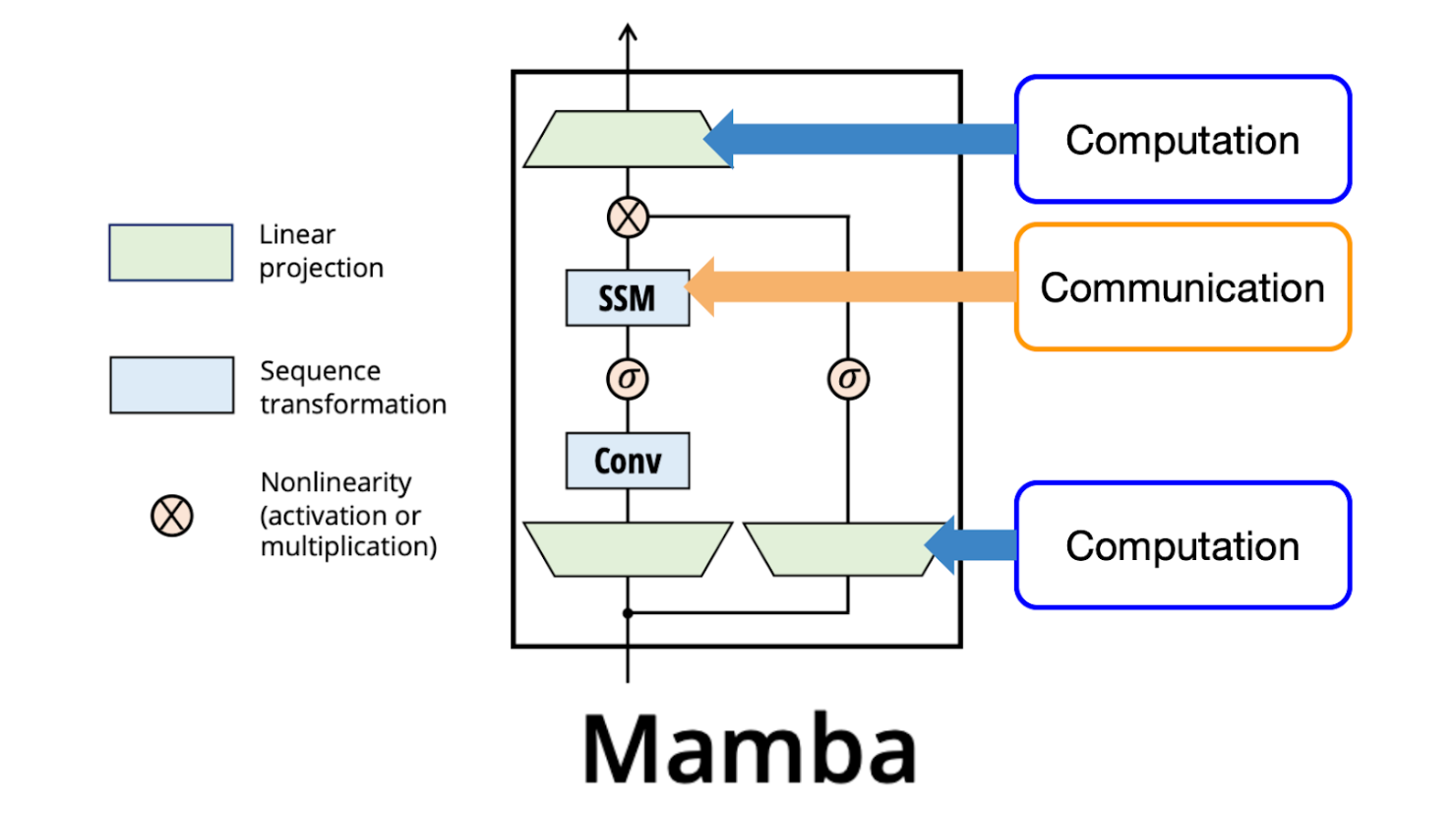
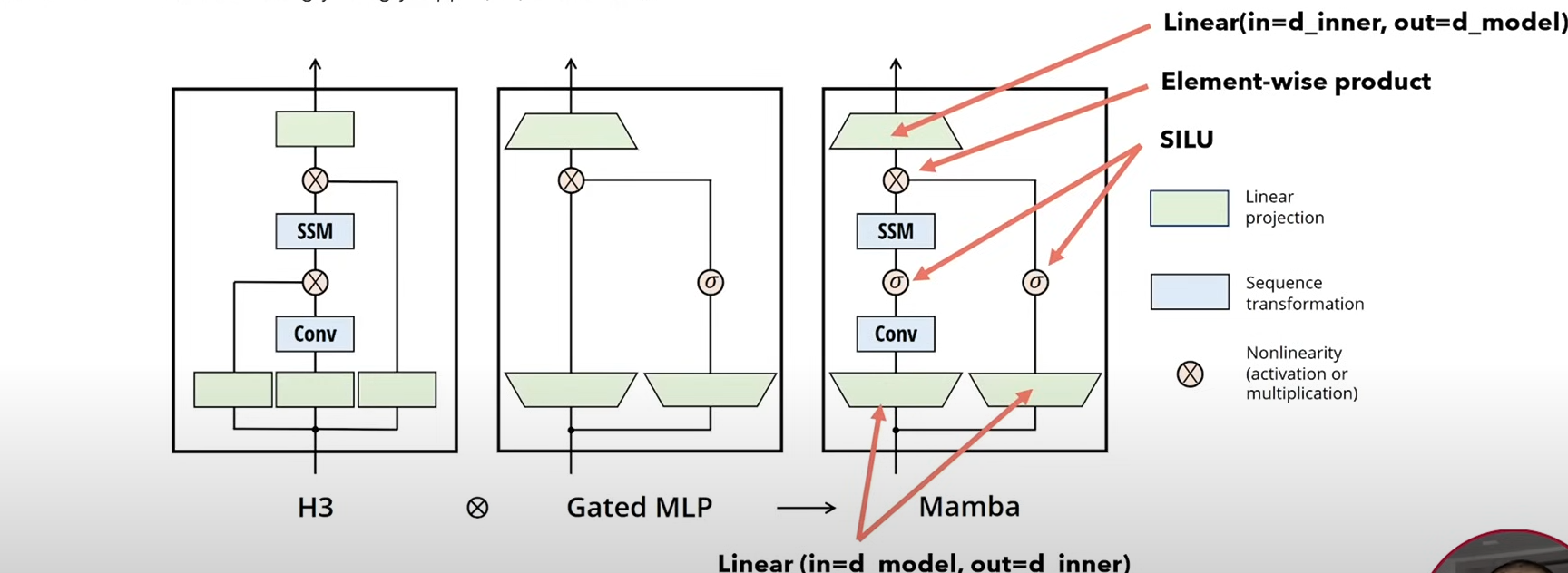
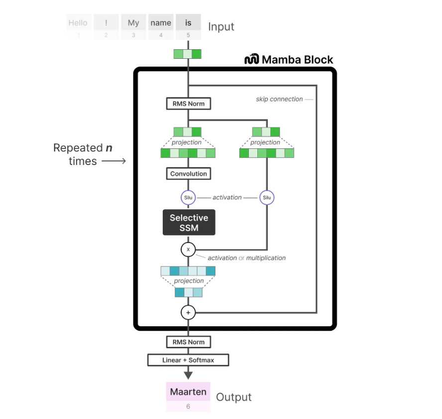
aside from the time-dependent $B, C, \Delta$, the Mamba block is a simplified H3 block:
- H3 used two SSMs - SSM-Shift (fixed, non-learned $A$) and SSM-Diag - so only $B, C$ were learnable inputs to the kernel. Mamba replaces the Shift SSM with a plain 1D convolution.
- H3’s query/key/value triad collapses into two projections (call them $q$ and $k$; the papers don’t, but the tutorial i worked from keeps the H3 naming).
- stacked blocks with no MLP interleaved between them.
a minimal implementation
a full one lives in HF transformers; here’s the tutorial version i walked. dimensions first:
@dataclass
class MambaConfig:
    state_size: int        # N - SSM state vector size
    hidden_size: int       # D - input embedding dim
    expansion_factor: int  # E - inner dim is E*D, like an MLP
    dt_rank: int           # R - rank of the delta projection (R << E*D)
    conv_kernel_size: int  # kernel of the 1D conv replacing SSM-Shift
three things to unpack: the block expands channels to $E \cdot D$ and projects back down at the output (MLP-style); $\Delta$ is first projected to a low rank $R$ before going to the inner dimension (cheap learned timescale, low-rank bottleneck); the 1D conv stands in for H3’s Shift SSM.
the outer block: two projections, a (causal) 1D conv, and a gate:
class Mamba(torch.nn.Module):
    def __init__(self, config: MambaConfig):
        super().__init__()
        self.state_size = config.state_size
        self.hidden_size = config.hidden_size * config.expansion_factor
        self.conv_kernel_size = config.conv_kernel_size

        self.conv = torch.nn.Conv1d(
            in_channels=self.hidden_size, out_channels=self.hidden_size,
            kernel_size=self.conv_kernel_size, padding=self.conv_kernel_size - 1,
            groups=self.hidden_size,      # depthwise
        )
        self.ssm = MambaSSM(config)

        self.q_proj = torch.nn.Linear(config.hidden_size, self.hidden_size, bias=False)
        self.k_proj = torch.nn.Linear(config.hidden_size, self.hidden_size, bias=False)
        self.out_proj = torch.nn.Linear(self.hidden_size, config.hidden_size, bias=False)

    def forward(self, input):
        sequence_length = input.shape[1]

        # 'hidden_states'/'gate' in HF; 'q'/'k' here for H3 consistency
        q = self.q_proj(input)
        k = self.k_proj(input)

        # pad k-1 on the left, cut to sequence length -> strictly causal conv
        conv_out = self.conv(k.transpose(1, 2))[..., :sequence_length]
        conv_out = torch.nn.functional.silu(conv_out)
        ssm_out = self.ssm(conv_out.transpose(1, 2))

        output = ssm_out * torch.nn.functional.silu(q)   # gated output
        return self.out_proj(output)
two details the minimal implementation glosses (and that i’ve added, because they cost me an afternoon):
- the gate: the output is
silu(q) ⊙ ssm_out. the $k$ branch (conv → silu → SSM) produces the content, the $q$ branch produces a per-channel valve on it. that’s the same in/out-projection shape H3 had, but the multiplication is an explicit gate. - the real reference implementation (mamba_simple.py) initializes
dt_proj’s bias to the softplus-inverse of a value drawn from $[10^{-3}, 10^{-1}]$, so the initial effective step sizes per channel land spread across that range instead of sitting in softplus’s flat near-zero region. minimal versions skip this; if yours trains badly, this is why.
inside the SSM - projections produce everything per-token, parameterization keeps $A$ decaying:
class MambaSSM(torch.nn.Module):
    def __init__(self, config: MambaConfig):
        super().__init__()
        self.hidden_size = config.hidden_size * config.expansion_factor
        self.state_size = config.state_size

        self.dt_proj_in  = torch.nn.Linear(self.hidden_size, config.dt_rank, bias=False)
        self.dt_proj_out = torch.nn.Linear(config.dt_rank,  self.hidden_size, bias=True)

        self.B_proj = torch.nn.Linear(self.hidden_size, self.state_size, bias=False)
        self.C_proj = torch.nn.Linear(self.hidden_size, self.state_size, bias=False)
        self.D = torch.nn.Parameter(torch.randn(self.hidden_size))

        A = torch.arange(1, self.state_size + 1).repeat(self.hidden_size, 1).float()
        self.A = torch.nn.Parameter(torch.log(A))

    def forward(self, input):
        batch_size, sequence_length = input.shape[0], input.shape[1]

        A = -torch.exp(self.A)   # (h, N) - negative real by construction, like S4D's log trick
        B = self.B_proj(input)   # (b, L, N)
        C = self.C_proj(input)   # (b, L, N)

        dt = self.dt_proj_out(self.dt_proj_in(input))
        dt = torch.nn.functional.softplus(dt)   # (b, L, h) - positive step sizes

        A_discrete = torch.exp(
            A.view(1, 1, self.hidden_size, self.state_size) *
            dt.view(batch_size, sequence_length, self.hidden_size, 1)
        )   # exp(dt * A), zero-order hold
        B_discrete = (
            B.view(batch_size, sequence_length, 1, self.state_size) *
            dt.view(batch_size, sequence_length, self.hidden_size, 1)
        )   # dt * B, the simplified (non-ZOH-exact) approximation
        ...
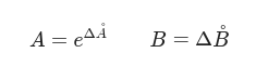
discretization here is ZOH-flavored, not bilinear like S4: $\bar{A}\cdot\bar{B} = e^{\Delta A}$ and $\bar{B} = \Delta B$. note the simplification: true ZOH computes $\bar{B} = A^{-1}(e^{\Delta A} - I)B$; the Mamba authors chose $\Delta B$ because it produced similar results (issue #19).
finally the recurrence itself - and this is the structural consequence of selectivity:
    ...
    outputs = []
    x = torch.zeros(batch_size, self.hidden_size, self.state_size)
    for i in range(sequence_length):
        current_input = input[:, i, :]

        # time-variant: every step gets its own parameters
        current_A_discrete = A_discrete[:, i, :, :]
        current_B_discrete = B_discrete[:, i, :, :]
        current_C = C[:, i, :]

        Ax = torch.einsum('bhn, bhn -> bhn', current_A_discrete, x)
        Bu = torch.einsum('bhn, bh -> bhn', current_B_discrete, current_input)
        x = Ax + Bu

        Cx = torch.einsum('bnx, bhn -> bh', current_C.unsqueeze(-1), x)
        Du = torch.einsum('h, bh -> bh', self.D, current_input)
        y = Cx + Du
        outputs.append(y)
    return torch.stack(outputs, dim=1)
the convolution view - the thing LSSL, S4 and H3 all used to parallelize training - dies here. the kernel $\bar{K}$ assumed $A, B$ fixed across positions; now every step has its own. the next section is the fix.
why selective at all
the motivation is two tasks time-invariant SSMs fail: selective copying (copy some tokens, ignore others) and induction heads (recall-and-repeat patterns). both need content-aware filtering, and fixed $A, B, C$ are static machinery - they spread everything through the state with the same weighting forever.
instead of fixed matrices, make $B$, $C$ and even the step size $\Delta$ functions of the input (shape-wise, the parameters pick up the sequence/batch dims):
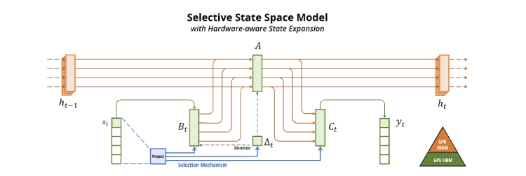
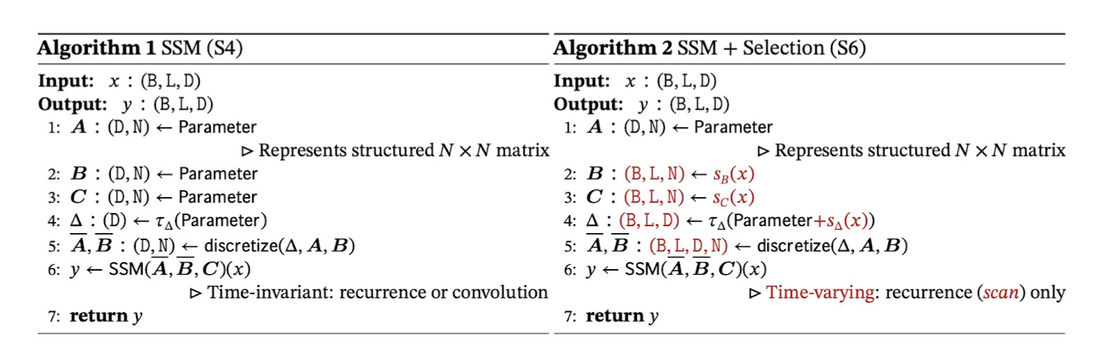
$B, C$ and $\Delta$ are learned per token - the $L$ in the $(B, L, N)$ shapes is exactly what makes it time-variant. one crucial constraint from the paper: $A$ stays input-independent. the state itself remains a static container; what drives into it ($B$) and reads out of it ($C$) becomes dynamic.
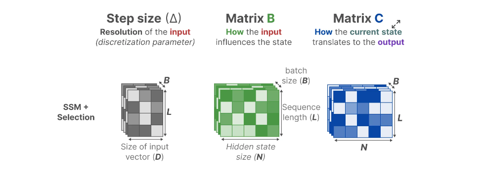
and $\Delta$ gets a physical read: a small step size means “mostly trust the accumulated context, ignore this token”; a large one means “focus on this token more than the context”. $\Delta$ is per-token attention-over-time, basically.

so this gets both worlds at once - selective about what enters the state (effectiveness vs plain SSMs) while the state stays bounded, $O(1)$ space per step and $O(n)$ total time (efficiency vs transformers). the paper’s own phrasing:
the efficiency vs. effectiveness tradeoff of sequence models is characterized by how well they compress their state: efficient models must have a small state, while effective models must have a state that contains all necessary information from the context. in turn, we propose that a fundamental principle for building sequence models is selectivity: or the context-aware ability to focus on or filter out inputs into a sequential state.
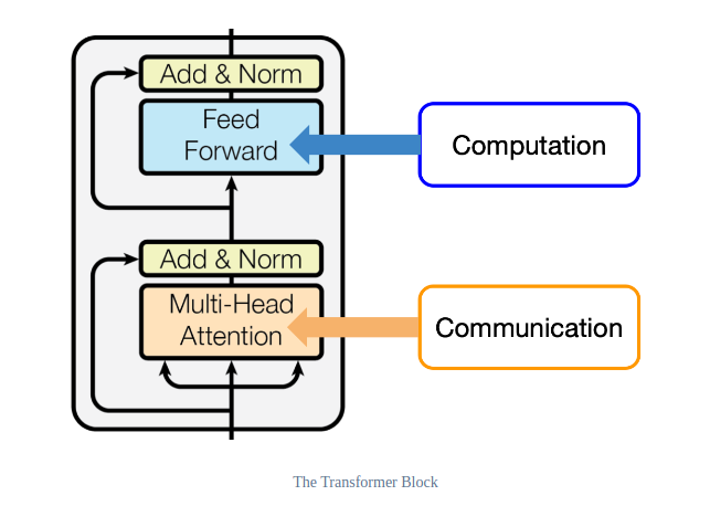
framing note that keeps the design legible: every good backbone does two things - communication between tokens and computation within a token. transformers do communication with attention, computation with MLPs; Mamba substitutes the SSM for the communication part and keeps MLP-style projections for computation.
the paper’s abstract, on results: “[Mamba] enjoys fast inference and linear scaling in sequence length, and its performance improves on real data up to million-length sequences… on language modelling, our Mamba-3B model outperforms Transformers of the same size and matches Transformers twice its size, both in pretraining and downstream evaluation.”
the two contributions
- a selective scan algorithm - the model can filter (ir)relevant information, and
- a hardware-aware algorithm - efficient storage of intermediate results via parallel scan, kernel fusion, and recomputation.
the gpu recipe
almost every GPU program: load data host DRAM → GPU HBM → GPU SRAM, compute, write back SRAM → HBM → DRAM. loading is by far the slowest leg; minimize it even at the cost of extra compute.
Tri Dao (Mamba co-author) earned his name on FlashAttention, which applied exactly this to self-attention: the intermediate $O(L^2)$ $QK^T$ matrix dwarfs the $O(L)$ inputs/outputs, so keep it in SRAM, tile over it, never round-trip it through HBM. Mamba applies the same playbook to the selective scan.
parallel scan, or making the recurrence parallel again
with time-variant parameters, the convolution form is gone and the recurrence looks irreducibly serial - state $t$ needs state $t-1$. the escape hatch: the update is associative. define the pair operator $a \otimes b$ over $(A_i, Bx_i)$-style first-order recurrence terms; recurrence composition is associative, $A * (B * C) = (A * B) * C$, so the sequence can be split into chunks, scanned in parallel, and combined:
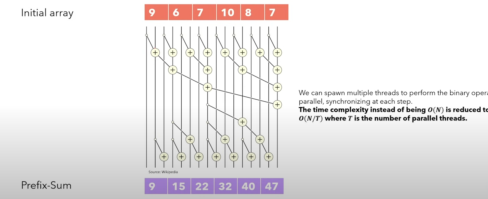
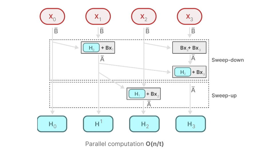
the concrete algorithm is the Blelloch work-efficient scan: first an upsweep (parallel reduction over a binary tree),
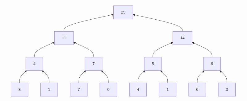
then a downsweep maintaining the invariant “every node holds the sum of all prior leaves” in pre-order traversal:
downsweep[N].left.value = downsweep[N].valuedownsweep[N].right.value = downsweep[N].value + upsweep[N].left.value
(blue = parent’s contribution; in the full tree, red = downsweep, yellow = upsweep, orange = combined.)
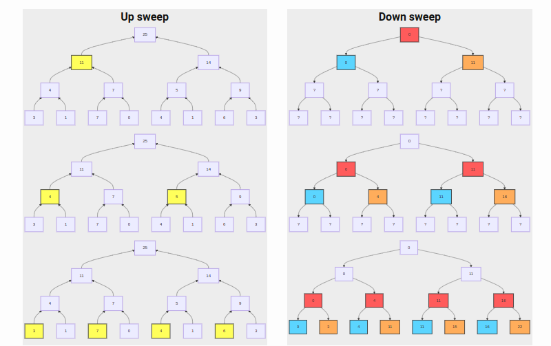
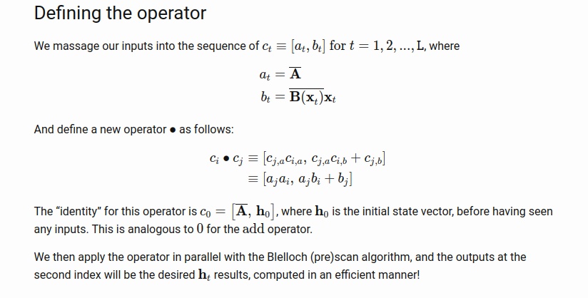
implemented in the reference kernel at selective_scan_common.h; jax.lax.associative_scan is a batteries-included version of the same Blelloch algorithm. time complexity drops from sequential $O(L)$ depth to tree $O(\log L)$ depth at the cost of more total FLOPs - the trade you want on a GPU.
dynamic $B$, $C$ + parallel scan = selective scan: time-variant and fast. hence the model’s alias S6 - an S4 computed with the selective scan.
kernel fusion + recomputation
like FlashAttention, Mamba minimizes DRAM↔SRAM round trips with kernel fusion: discretization ($\Delta$), the selective scan, and the multiplication with $C$ all run inside one kernel, never materializing intermediates in HBM.
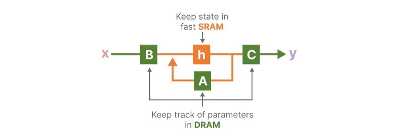
the last piece is recomputation: the intermediate states (needed for the backward pass) are not stored; during backprop, inputs are re-loaded from HBM to SRAM and states are recomputed on the fly. SRAM is fast, so recomputing beats storing-and-loading - which is how the selective scan ends up with the same memory requirements as a FlashAttention-grade transformer implementation.
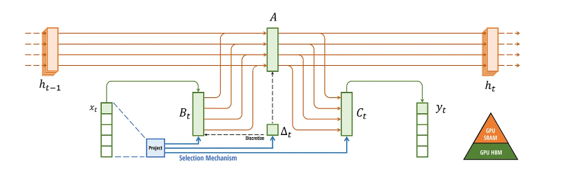
the resulting model, summed up
the selective SSM = recurrent SSM via discretization + HiPPO init on $A$ for long range (S4 heritage) + selective scan for compression + hardware-aware algorithm for speed.
papers & sources
- Mamba: https://arxiv.org/abs/2312.00752
- Mamba-2 / SSD (state duality - read next): https://tridao.me/blog/2024/mamba2-part1-model
- reference impl: https://github.com/state-spaces/mamba, HF: modeling_mamba.py
- selective copy / induction-head tasks paper: https://arxiv.org/abs/2310.15449
- my SegMamba notes - first place SSMs hit my actual domain (3D medical segmentation)
todos
- write the selective-scan math out properly: first-order recurrence pairs, the composition operator, and the proof sketch of associativity. the images above carry it; the text still doesn’t.
- Mamba-2: the SSD formulation collapses the scan into a structured matrix multiply and ditches the SSM/attention dichotomy (state duality). the blog link is queued; read the series.
- collect the actual benchmark tables (LRA / language / audio) into this note - my earlier copy leaned on the abstract’s claims instead of numbers.