

S4 notes
S4 in one line: SSM + optimized HiPPO + structured matrices. this note walks from the LSSL lead-in, through the diagonalization story, to the S4 kernel trick and the simplifications that came after (S4D init, LRU). builds directly on SSM notes and HiPPO notes - keep the hippo_matrix() cell from the latter in reach, it gets reused here. main sources: annotated S4, Albert Gu’s Stanford talk and interview, the visual guide.
before S4: LSSL, one layer with three hats
Gu et al 2021: the Linear State-Space Layer maps a 1-D input/sequence $u(t) \to y(t)$ through an implicit state $x(t)$, by simulating a linear continuous-time SSM in discrete time.
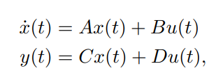
the one layer, seen from three angles:
- recurrent: fix $\Delta t$ and discretize into a linear recurrence; inference runs stateful with constant memory and compute per step.
- convolutional: LTI systems are explicitly representable as a continuous convolution, and the discrete version trains in parallel as a convolution.
- continuous-time: the layer is a differential equation, so it does continuous-time tricks - simulate continuous processes, handle missing data, adapt to timescales.
generality has a price, and the paper names both: (i) naive LSSLs inherit the long-dependency limits of both RNNs and CNNs, and (ii) the state matrix $A$ and timescale $\Delta t$ are critical to performance, yet learning them is computationally infeasible. the fix is the part that matters: specialize $A$ to a class of structured matrices that generalize the continuous-time memory theory - i.e. HiPPO - and give algorithms that make learning such an $A$ tractable.
step 1 - make A diagonal, legally
from HiPPO we have a matrix that remembers everything, but it’s dense - $O(N^2)$ matvecs. the search S4 runs: a matrix that’s diagonal, yet still effective at preserving information across many timesteps. diagonal means $O(N)$ matvecs and a kernel you can compute cheaply.
the legal move is a similarity transform.
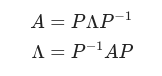
a matrix is diagonalizable if $A = P\Lambda P^{-1}$ for some diagonal $\Lambda$ and invertible $P$. now define a new state vector $\tilde{x} = Px$ - a pure change of coordinates:
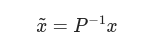
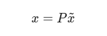

substitute everywhere and the SSM keeps its input-output behavior exactly, with rewritten parameters:


we didn’t change the model, we changed the basis it lives in. so: diagonalize the HiPPO matrix, enjoy $O(N)$…
step 2 - and watch the diagonalization blow up
from sympy import Matrix

A = Matrix(hippo_matrix(state_size=16))
P, Lambda = A.diagonalize()      # A = P @ Lambda @ P^-1
Pinv = P.inv()

# sympy works exact; split into real/imag parts to see the scale
P_real, Pinv_real = P.as_real_imag()[0], Pinv.as_real_imag()[0]
max_value = max([max(P_real), max(Pinv_real)])
print(f"Max Value: {max_value:.3f}")
# Max Value: 4390273247.525
at state size 16, the entries of $P$ and $P^{-1}$ already reach ~$4.4\times10^9$, and they grow exponentially with $N$. $P$ is the poison: $P\Lambda P^{-1}$ has to be formed with those magnitudes, so the “equivalence” is numerically worthless. dense-but-stable vs diagonal-but-exploding - classic.
side note that the code above forces you to learn: these $P$/$\Lambda$ are generally complex ($\alpha + \beta i$). that’s why reference S4/S4D implementations store parameters in torch.cfloat:
import torch
t = torch.randn(3, dtype=torch.cfloat)
print(f"Element Size: {t.element_size() * 8} bits")
# Element Size: 64 bits
each cfloat value is two floats (real + imaginary), 64 bits total.
step 3 - S4D-Lin: just pick a good diagonal directly
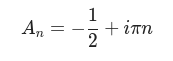
S4D (parameterization and initialization of diagonal SSMs) skips the dance: derive a specific diagonal $A$ that approximates HiPPO’s behavior. the flavor used here, S4D-Lin, puts $-\tfrac12$ on the real part of every diagonal entry (so every mode decays) and grows the imaginary part linearly (so modes oscillate at distinct frequencies):
import math, torch
state_size = 4
s4d_lin_A = torch.tensor([-0.5 + (math.pi * n * 1j) for n in range(state_size)])
print(torch.diag_embed(s4d_lin_A))
watch the sign: the real parts must stay negative. positive real part = modes that grow = instability, and during training $A$ can drift positive. the S4D trick is to parameterize the log of the real part so the network can only ever produce a decaying diagonal:
def __init__(self, state_size):
    ...
    A = s4d_lin_initialization(state_size)
    self.log_A_real = torch.nn.Parameter(torch.log(-A.real))
    self.A_imag = torch.nn.Parameter(A.imag)
    ...

def forward(self, input):
    A = -torch.exp(self.log_A_real) + 1j * self.A_imag
    ...
initialize at log(1/2), recover $A$ as $-\exp(\cdot) + i\,\text{imag}$. negative forever, by construction. (the -A.real inside the log matters: a naive transcription logs the already-negative value, and torch.log of a negative is NaN. the reference repo’s log_A_real holds $\log\lvert{\rm Re}\,A\rvert$.)
the convolution view, or: SSMs are CNNs with an infinite window
the thing S4 actually speeds up is kernel $K$ = the convolution-form SSM from my SSM notes ($y = \bar{K} * x$, $\bar{K}_j = C\bar{A}^j\bar{B}$).
an intuition that stuck with me: an exponential moving average is nothing but convolving the input with an exponentially decaying kernel. that’s a tiny SSM: one channel, $\bar{A} = $ scalar decay. a CNN is the same shape but with a finite learned window; the SSM kernel decays forever. SSM = CNN with an infinitely long context window, run online as a recurrence at inference.
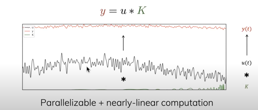
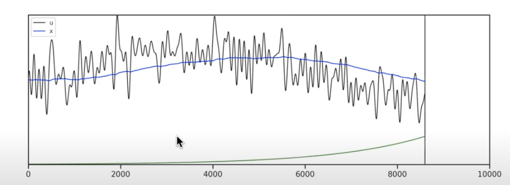
and the composition that defines S4: state space models + HiPPO for long-range dependencies + discretization to get the recurrent and convolution representations. two empirical notes from the visual guide worth keeping: random initialization with S4 gives middling performance - the HiPPO init mattered for S4; and S4D-style init carries over to Mamba nicely, though there random init also works well. hold that asymmetry, it gets resolved in the LRU section.
the state is bigger than the input - here’s the deal
one subtlety: the input $x$ is a 1-D signal per channel, the state $h$ is $N$-dimensional (HiPPO’s $N$ coefficients). so the layer expands the channel into an $N$-dim compressed history, and then $C$ reads it back down to 1-D output per channel. why expand at all only to condense? because a multi-dimensional input scenario wants many states each capturing different parts of the input dynamically - i.e. each channel gets its own SSM and its own tiny memory:
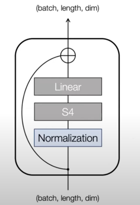
cost math: input length $L$ means $O(L)$ sequential computation for the recurrent form - linear, no quadratic token-token attention. the matvec inside each step is the real cost driver, and that’s where the structured/diagonal $A$ pays off. (my earlier note claimed the state is “100x the input size” - that number was made up; the state expansion $N$ is a hyperparameter, S4 used up to a few hundred.)
regime note: transformers are great for dense discrete data (language); S4 loves noisy, raw, continuous-ish signals (audio, sensor streams).
everything so far is LTI - and here comes Mamba
to be crisp about the boundary (this sentence is easy to read backwards: Mamba’s change is relative to S4 - it just removes linear time invariance):
- S4/S4D: $\bar{A}, \bar{B}, \bar{C}$ fixed for every timestep. static. content-blind.
- Mamba: $B, C, \Delta$ become functions of the input $x_t$. selectivity.
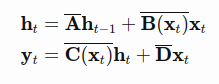
with time-variance, the model stops learning fixed matrices and learns functions that ingest the input and then control the output dynamics.
the DPLR kernel (the actual S4 contribution, kept as a headline)
S4’s speed contribution: a stable method for computing $K$ when $A$ has diagonal plus low-rank (DPLR) structure in complex space:
\[A = \Lambda - PQ^* \qquad \Lambda \text{ diagonal}, \quad P, Q \in \mathbb{C}^{N\times 1}\](rank-1 without loss of generality - and this is the exact shape of the diagonalized HiPPO matrix, which is the whole point: HiPPO’s unstable $P$ gets absorbed into a low-rank term instead of a dense similarity transform). three steps, as in annotated S4:
- don’t compute $K$ directly; compute its spectrum via the truncated generating function $\tilde{K}(z) = \sum_k \overline{K_k} z^k$ - the powers $\bar{A}^k$ turn into a matrix inverse $\left(\tfrac{1}{z} - \bar{A}\right)^{-1}$-shaped object.
- the diagonal part of that inverse evaluates as a Cauchy kernel: entries $\tfrac{1}{\omega_j - \zeta_k}$, computable with a handful of FFTs.
- the low-rank correction $\left(\Lambda - PQ^\right)^{-1}$ gets Woodbury’d back to diagonal scale: $\left(\Lambda - PQ^\right)^{-1} = \Lambda^{-1} + \Lambda^{-1}P\left(I - Q^\Lambda^{-1}P\right)^{-1}Q^\Lambda^{-1}$. (sign trap: secondary notes sometimes print this with a plus; the S4 convention is $\Lambda - PQ^*$ throughout.)
after all that math, the implementation is four functions: K_gen_DPLR (generating function for DPLR $A$), conv_from_gen (gens → filter), causal_convolution (run it), discretize_DPLR (SSM → discrete RNN form).
revisit owed: the full derivations - annotated S4 part 2 and annotated Mamba (hard version). generating functions + Cauchy matrices need proper groundwork first.
coda: simplifications that followed (LRU, S5)
Orvieto et al 2023 (“Resurrecting RNNs for Long Sequences”) lands the uncomfortable observation: S4 looked theoretically principled - continuous-time inspiration, HiPPO-based init, careful discretization - but follow-ups (DSS, S4D, S5) suggested the specific HiPPO initialization is often not crucial for performance, and the discretization rules that actually perform best deviate from the theory. so what is doing the work, mechanistically? nobody quite knew.
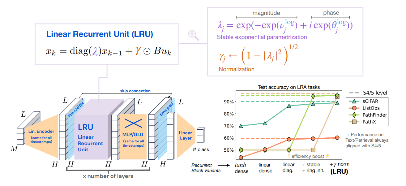
their answer: strip it to a Linear Recurrence Unit - complex-diagonal recurrence with a parameterization that provably keeps the decay factor inside the unit circle (signals don’t explode/vanish), wrapped in a stack of LRU blocks with nonlinear projections, skip connections and batch/layer norm between them. matches S4-scale results on the Long Range Arena with a tiny fraction of the machinery. the S5 line (Smith et al 2022) similarly cut S4 down to a single diagonal recurrence per layer run with a parallel scan.
so the arc is: S4 needed HiPPO to work at all → S4D made the structure explicit and trainable → LRU showed the linear recurrence with stable parameterization is the load-bearing part, not the control-theory pedigree. Mamba then bet the other direction (make it input-dependent, keep the hardware-aware scan) - and won the popularity contest.
papers & sources
- S4: https://arxiv.org/abs/2111.00396 - structured dense matrix vector mult lineage: https://arxiv.org/pdf/1611.01569
- DSS: https://arxiv.org/abs/2203.14343, S4D: https://arxiv.org/abs/2206.11893, S5: https://arxiv.org/abs/2208.04933, LRU: https://arxiv.org/abs/2303.06349
- annotated S4 - Albert Gu’s Stanford talk, interview - visual guide
todos
- derive the DPLR kernel properly (generating function → Cauchy → Woodbury) instead of reading it as three magic nouns. prerequisites: differential equations, complex analysis basics.
- reconcile the HiPPO-init story across years: S4 papers “init is critical” vs LRU “init barely matters”. i suspect the answer is “critical then, not now, because normalization/parameterization grew up” - worth 30 minutes with the LRU ablations.
- walk the Annotated S4 sympy instability experiment again and note at which $N$ the $P$ entries cross 10^k thresholds - it’s the cleanest motivation for S4D there is.