

HiPPO notes
in my SSM notes the whole thing came down to one line: the structure of $A$ decides which parts of the previous state survive. HiPPO (“High-order Polynomial Projection Operators”, paper, Gu, Dao, Ermon, Rudra, Ré) is the answer to “so what should $A$ be?” - and it’s not a trick, it’s a whole framework: project the entire input history onto a space of polynomial coefficients, online, with closed-form update matrices. this walkthrough follows the Hazy Research blog, the paper itself, Yao Fu’s post, and Albert Gu’s talk.
why A is the whole ballgame
in the recurrent view, $h_k = \bar{A}h_{k-1} + \bar{B}x_k$, the state can only look back at the previous state. nothing else survives. so $A$ is the difference between remembering a few tokens and capturing everything seen thus far.
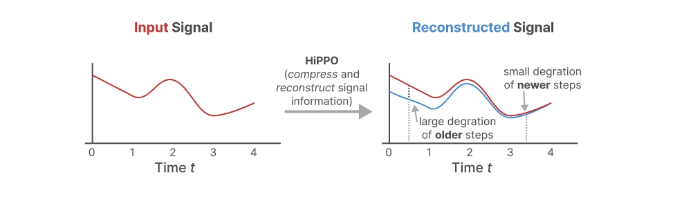
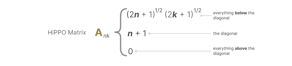
the idea in one sentence: compress all input seen so far into a fixed vector of coefficients, where $A$ is built so recent tokens are sharp and older ones fade in a principled way.
the operator in one cell
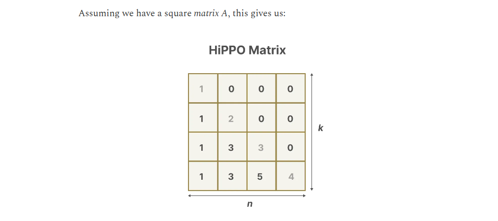
here’s the LegS matrix spelled out (I’ll show where it comes from below), producing the right values for $N = 5$:
import torch

def hippo_matrix(state_size):
    # diagonal is -(1, 2, ..., N)
    A = torch.diag(torch.arange(1, state_size + 1, dtype=torch.float))

    def lower(n, k):
        return (2*n + 1)**0.5 * (2*k + 1)**0.5

    for i in range(1, state_size):
        for j in range(i):
            A[i, j] = lower(i, j)

    return -1 * A

hippo_matrix(state_size=5)
# tensor([[-1.0000, -0.0000, -0.0000, -0.0000, -0.0000],
#         [-1.7321, -2.0000, -0.0000, -0.0000, -0.0000],
#         [-2.2361, -3.8730, -3.0000, -0.0000, -0.0000],
#         [-2.6458, -4.5826, -5.9161, -4.0000, -0.0000],
#         [-3.0000, -5.1962, -6.7082, -7.9373, -5.0000]])
lower-triangular, negative, diagonal exactly $-n$: each coefficient slides toward zero at its own rate. (keep this cell in your head - my S4 notes diagonalize this matrix.)
the actual problem
popular models suffer from forgetting: attention has a fixed-size context, RNNs have vanishing-gradient-limited memory horizons. HiPPO attacks the fundamental version of this: incrementally maintaining a memory representation of sequences from first principles.
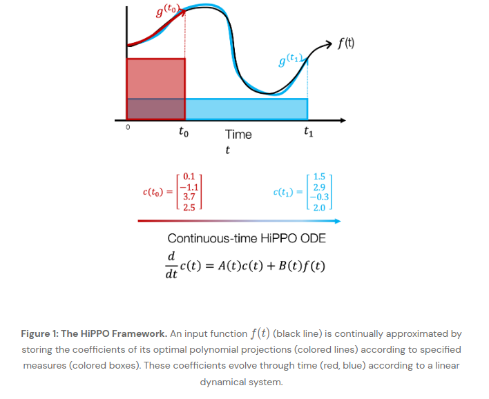
the setup from the paper: given input $f(t)$ we need its cumulative history $f_{\le t}$ at every $t$, but the space of functions is too big to memorize - so we project onto a subspace of bounded dimension $N$. two ingredients define the problem fully:
- a way to quantify approximation - a probability measure $\mu$ on $[0, \infty)$ defines the inner product $\langle f, g \rangle_\mu = \int_0^\infty f(x)\, g(x)\, d\mu(x)$, a Hilbert space, and a norm $\lVert f \rVert_{L_2(\mu)} = \langle f, f \rangle_\mu^{1/2}$. since we only ever have $f_{\le t}$, the measure must vary with time: $\mu^{(t)}$ supported on $(-\infty, t]$. the measure controls which parts of the history matter.
- a subspace $G$ of dimension $N$ - $N$ is the approximation order, i.e. the size of the compression; the projected history is $N$ coefficients in any basis of $G$. the degree of the polynomial, i.e. the number of coefficients, is literally the memory budget.
so the two essential questions:
- how do I calculate a state $x(t)$ that encodes the history of the input up to time $t$?
- how do I update that state online as new input keeps arriving?
and the design dial: the measure lets you pick the decay behavior - weigh the recent past more than the far past (sliding-window-ish), or treat the whole span uniformly. HiPPO’s headline measure (LegS) does the second: full history, no sliding window.
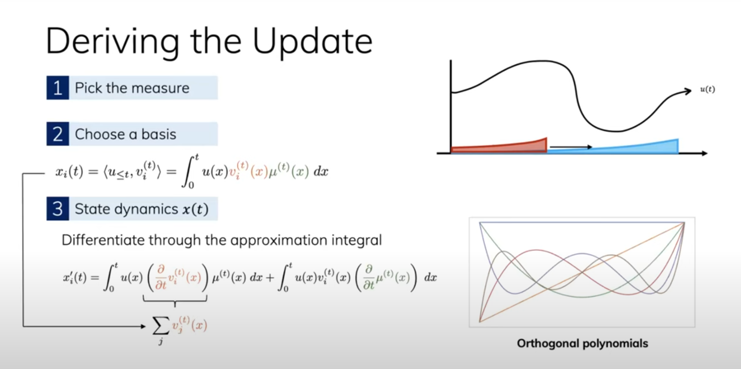
step 1 - pick the measure (hyperparameter; could even be learned, that’s an open idea). the framework then hands you closed-form transition matrices $A(t), B(t)$ that optimally track the approximation under that measure.
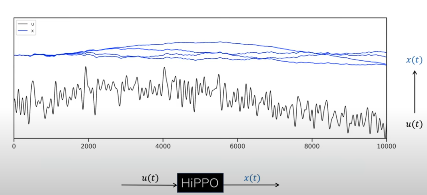
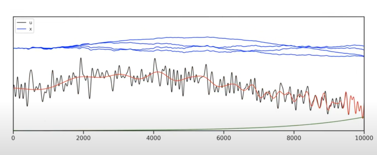
the part that genuinely amazed me: at any instant, all you have is the coefficient vector - the state - and HiPPO can reconstruct the whole input history up to now from it. the state is a lossy ZIP of everything you’ve ever seen.
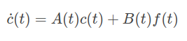
for the practitioner: maintain a memory $c_t$ of input $f_t$ via the linear recurrence $c_{t+1} = A_t c_t + B_t f_t$ with closed-form $A_t, B_t$. that’s it.
plugging it into an mlp/rnn
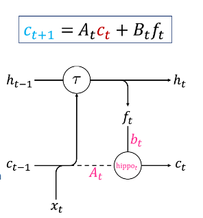
- start with a standard recurrence $h_t = \tau(h_{t-1}, x_t)$ with any nonlinear $\tau$; project the state down to a smaller feature $f_t$;
- run the HiPPO recurrence on $f_t$ to keep the compressed history $c_t$;
- feed $c_t$ back into $\tau$.
the math walk
this section roughly follows Yao Fu’s post; section pointers refer to the HiPPO paper.
encode a function by linear approximation (≈ sec 2.1)
functional analysis is linear algebra where the vector space is a space of functions. any $f(t)$ can be a linear combination of basis functions $e_i(t)$:
\[f(t) = \sum_{i=1}^{\infty} c_i\, e_i(t)\]infinite basis - unusable. truncate to $N$ (less error the bigger the $N$), and the approximation is $\hat{f}(t) = \sum_{i=1}^N c_i e_i(t)$, with the coefficients found by least squares exactly like in linear algebra. want $f$ at any $\tau$? evaluate $\sum_i c_i e_i(\tau)$. the coefficients are the information.
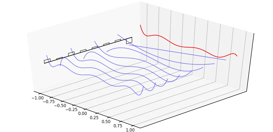
this will become the hidden state of a special RNN, updated online by the HiPPO matrix.
a note on why Legendre polynomials specifically: consecutive orders capture progressively finer structure (low order = general trend), they’re orthogonal (each basis function carries independent signal features - no redundancy, stable numerics), and they’re cheap to compute recursively. orthogonal basis + online projection = the right tool for compactly approximating smooth-ish signals.
find the coefficients by solving an ODE (≈ sec 2.1-2.2)
the coefficients come from the inner product of the target against each basis function, under the measure:
\[c_i(t) = \langle f_{<t}(x), e_i(x) \rangle_\mu := \int_0^\infty f_{<t}(x)\, e_i(x)\, d\mu(x)\]differentiate that for every $i$, push through (a large amount of) math, and the integral drops out - the coefficients satisfy an ODE (paper appendix D.3):
\[\frac{d}{dt}c(t) = -\frac{1}{t}Ac(t) + \frac{1}{t}Bf(t)\]with $c(t) = [c_1(t), \dots, c_N(t)]$. and here the magic matrix $A$ emerges (it’s HiPPO’s matrix first - the S4 paper adopts it later, which is why my S4 notes start from here):
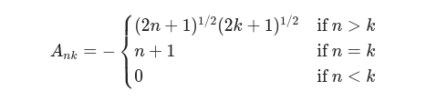
\[A_{nk} = \begin{cases} (2n+1)^{1/2} (2k+1)^{1/2} & \text{if } n > k \\ n+1 & \text{if } n = k \\ 0 & \text{if } n < k \end{cases}\]exactly the matrix computed by hippo_matrix() above. the derivation sketch: differentiate $c_i(t)$ w.r.t. $t$ (appendix C.3), eliminate the integral using the recurrence relations of Legendre polynomials (appendix B.1.1 + D.3), vectorize the resulting ODEs - $A$ falls out at that step.
scale the basis as time grows (sec 3) → LegS
problem: the basis lives on a fixed domain, time doesn’t stop. fix: dynamically rescale the basis to always cover $[0, t]$.
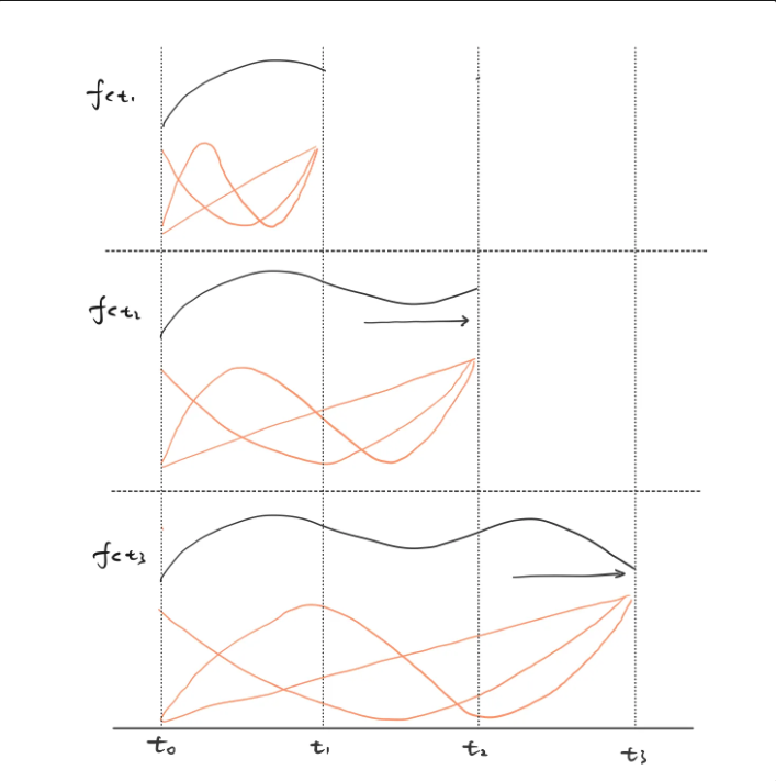
formally, define the scaled Legendre measure:
\[\mu^{(t)} = \frac{1}{t}\mathbb{1}_{[0,t]}\](uniform over everything seen so far - this is the “keep the full history, not a sliding window” choice, and it’s why HiPPO needs no sequence-length priors; LegS generalizes across timescales). the general recipe:
- pick a measure $\mu^{(t)}$;
- it induces an inner product;
- Gram-Schmidt under that inner product induces the polynomial basis - here, automatically scaled to $[0, t]$.
plug measure + inner product + basis into the ODE, get the LegS matrix $A$ (appendix B.1 + D.3).
discretize the ODE → an RNN (sec 2.4)
the payoff, straight from the paper: the ODE dynamics consume the sequence, and discretization turns them into an RNN:
\[\text{before: } \frac{d}{dt}c(t) = -\frac{1}{t}Ac(t) + \frac{1}{t}Bf(t) \qquad \text{after: } c_{k+1} = \left(1 - \frac{A}{k}\right)c_k + \frac{1}{k}Bf_k\](i) consume input sequence ${f_k}$, (ii) implicitly define $f(t)$ with $f(k\Delta t) = f_k$, (iii) evolve $c(t)$ through the ODE, (iv) sample back $c_k := c(k\Delta t)$
and these $c_k$ are exactly the coefficients of the online approximation at time $k\Delta t$:
\[\hat{f}_{<k\Delta t}(x) = \sum_{i=1}^N c_{k,i}\, e_{k\Delta t, i}(x)\]so the state of this RNN is never just “some numbers” - it’s a live polynomial approximation of the entire past, and the recurrence is the compression algorithm. this is the thing S4 runs with (structured + diagonalized), and Mamba mutates (selective - my Mamba notes. linear recurrence, closed form, all of history. that’s the whole trick.
todos
- actually walk appendix D.3 - i still trust the ODE more than derive it. needs the ODE/Legendre-recurrence groundwork first.
- the measure zoo: the paper has LegS (scaled uniform) but also LagT/LegT sliding-window flavors. what does each buy, and which one does S4/Mamba actually inherit? (S4’s init is LegS-derived; the LRU line says init barely matters - check against my S4 notes.)
- “measure as a learned dynamic parameter” instead of a fixed choice - nobody in the papers does this; worth a skim of follow-up work.