


Information Retrieval notes
built from my own information-retrieval readme, plus the kmwllc BM25 walkthrough.
IR in its most basic form answers: how relevant is a given query for a document? the catch is scale - not one document but millions or billions, so the real question is how to find the relevant handful efficiently.
what counts as relevance
- a query has many words; a processing pipeline (below) breaks it into individual terms.
- a word appearing more often in a document signals relevance - so count occurrences.
- longer documents inflate raw counts - so document length must factor in.
- counting across the whole corpus at query time would be hopeless - so counts are stored before queries arrive, in a structure built for lookups.
the inverted index
the structure that makes retrieval feasible: precomputed term statistics, queryable by term.
- document frequency df_t: how many documents contain the term
- term frequency tf(t,d): how often the term appears in document d
- document length dl, and the corpus average document length adl
building it runs every document (and later, every query) through the same pipeline: tokenization -> stemming -> stop word removal.
- tokenization: split into individual terms.
- stemming: reduce words to roots before indexing. the crude version chops suffixes by heuristic (the classic: Porter’s algorithm, empirically effective since 1980); the expensive version, lemmatization, uses vocabulary + morphological analysis to map inflectional forms to the dictionary form (
am, are, is -> be,car's, cars -> car). the pipeline’s net effect on text:the boy's cars are different colors -> the boy car be differ color. - stop word removal: drop the most common words (articles, pronouns) that appear everywhere and discriminate nothing.
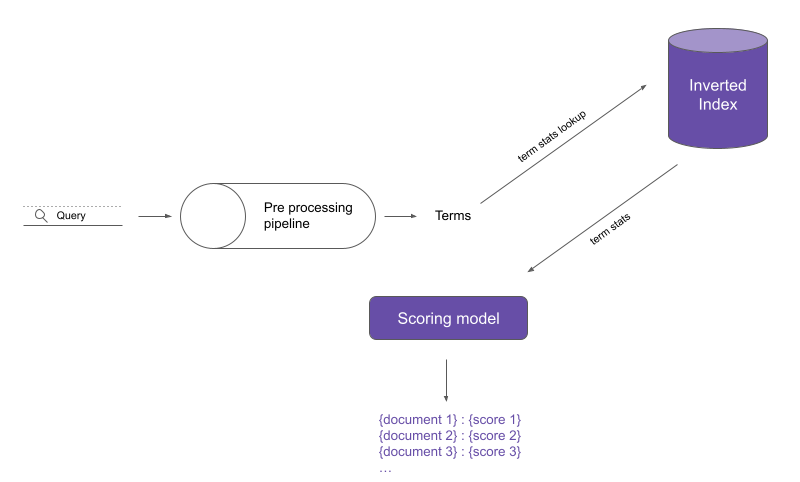
the honest limitation to carry: a document can be relevant without containing the exact query terms. classic IR can’t see past symbol identity - which is exactly the gap BERT-style semantic search later attacked.
scoring models, and their shared blindness
everything in this section treats terms as discrete symbols and documents as token streams - no meaning anywhere. keep that in mind while the math gets fancy.
tf-idf
\[TFIDF(q, d) = \sum_{t\;\in\;T_d \cap T_q} \log(1 + tf_{t,d}) \cdot \log\frac{\lvert D \rvert}{df_t}\]- term frequency: raw counts overshoot; dampen with
log(1 + tf(t,d))(or use relative frequency tf/dl - the medium-post form: TF = repetitions of the word in the document / words in the document). - inverse document frequency: the term’s “informativeness”: $\lvert D \rvert$ documents total, the term appears in
df_tof them, so $\log(\lvert D \rvert / df_t)$ is large exactly for terms that rarefy the document set.
why log in the IDF? two honest layers:
- the practical one: compresses a huge ratio range into a sane scale, and a term appearing in all documents ($df = \lvert D \rvert$) gets weight 0 rather than a tiny nonzero.
- the real one: IDF isn’t an ad-hoc scaling, it’s the derivative of the probabilistic retrieval model - the Robertson-Spärck Jones weight, which estimates the discrimination value of a term and comes out as a log of the odds ratio approximately equal to $\log(\lvert D \rvert / df_t)$ for rare terms. the “log prevents the numerator from blowing up” explanation is the pop version; the RSJ derivation is the thing to actually cite.
also: computing tf-idf as a full document×vocabulary matrix is how you’d think about it mathematically, but storage is the wall. 1 M documents × ~1000 terms each with a 100k vocabulary: the matrix is 10¹¹ cells with only ~10⁹ nonzero (each document touches 1000 of its 100,000 slots) - ~99% zeros (the ~90% you’ll see in places comes from an arithmetic slip: comparing the nonzero count against 90% of the matrix’s columns ignores that each row only has ~1000 nonzeros). store per-posting statistics in the inverted index instead, and only the nonzero cells exist.
BM25
the fix for tf-idf’s naivety about repetition. if a document says “elephant” 200 times, is it twice as relevant as one that says it 100 times? no - past some point the document is saturated with the term; further mentions add nothing. tf-idf keeps rewarding every extra occurrence, so the task becomes: reshape the TF term so its contribution rises fast at low tf and slows to a plateau as tf grows.
step 1 - term saturation. compress tf:
\[\frac{tf}{tf + k_1}\]small tf values rise quickly; the curve flattens toward 1 as tf grows. $k_1$ is the knob that sets where the plateau bites.
step 2 - document length. one “elephant” in a 50-word document is strong evidence; one in a 10,000-word document is nothing. so matches in short documents deserve more reward, and longer documents should need more occurrences for the same credit. the trick of step 1 does this implicitly if k grows with document length: make it
\[k_1 \cdot \frac{dl}{adl} = k_1 \cdot \frac{tf}{tf + k_1 \cdot dl/adl}\]shorter than average (dl/adl < 1) → smaller k → the plateau arrives sooner; longer than average → larger k → more occurrences tolerated before saturation. and a subtle bonus: a longer document now sits on a slower-saturating curve, exactly the intuition one wants.
step 3 - interpolate, don’t force. multiplying k by dl/adl unconditionally makes length matter 100%. real ranking needs a dial between “ignore length” and “full normalization”:
\[tf \,\cdot\; \big(1 - b + b \cdot \tfrac{dl}{adl}\big)\]- b = 0 → the multiplier is 1, length ignored;
- b = 1 → exactly the dl/adl scaling from step 2;
- in between → partial responsiveness as dl/adl varies.
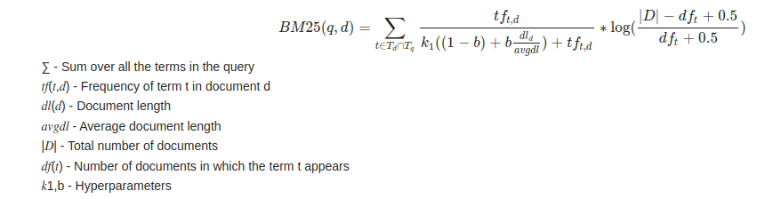
the assembled score (full BM25, IDF term included):
\[\text{score}(q, d) = \sum_{t \in T_q} \underbrace{\log\!\Big(\frac{N - df_t + 0.5}{df_t + 0.5} + 1\Big)}_{\text{IDF (RSJ-style, smoothed)}} \cdot \underbrace{\frac{tf(t,d)\,(k_1 + 1)}{tf(t,d) + k_1\,(1 - b + b\,\frac{dl}{adl})}}_{\text{saturating, length-normalized TF}}\]the (k₁+1) numerator is a scale factor so the term peaks near k₁+1 instead of near 1. the usual hyperparameter ranges: 1.2 < k_1 < 2, 0.5 < b < 0.8 - k₁ controls term-frequency saturation, b controls document-length normalization. the +0.5 smoothing in IDF keeps rare-term weights finite; the exact form varies by implementation (Lucene’s is the one above).
the “IDF arrived at to give deterministic results” phrasing, stated properly: it’s the Robertson-Spärck Jones probabilistic weight; i’ve left the derivation out here too.
word2vec (the dense-representation bridgehead)
word2vec is the bridgehead toward semantic search - the connection to everything above is a swap: replace the discrete-symbol assumption with dense vectors learned from context (the BERT-for-IR half is still a todo below).
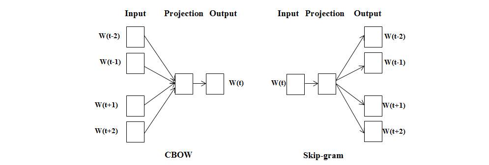
word2vec iterates over a corpus with a sliding window: at each step take a center word and its context words, softmax over the whole vocabulary, cross-entropy loss on the context words, backprop into the embeddings. two flavors: CBOW predicts the center from the context, skip-gram predicts the context from the center.
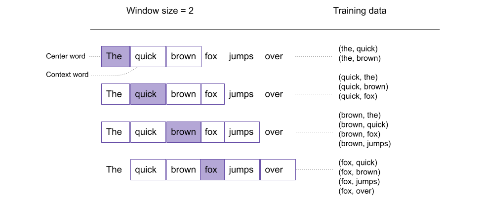
full notes live in my word2vec note - what matters for IR are the drawbacks, because they explain why BERT-class models took over retrieval:
- bag-of-words at heart: word order within the window is invisible
- small window ⇒ only very local context shapes a vector
- one vector per surface form: “river bank” and “bank deposit” collapse “bank” into a single embedding
- no handling for out-of-vocabulary words
sources
- my repo (the true source of this note): https://github.com/kuutsav/information-retrieval
- tf-idf & BM25 walkthrough: https://kmwllc.com/index.php/2020/03/20/understanding-tf-idf-and-bm-25/
- tf-idf explainer (medium): https://medium.com/analytics-vidhya/tf-idf-term-frequency-technique-easiest-explanation-for-text-classification-in-nlp-with-code-8ca3912e58c3
todos
- add the BERT-for-IR section: bi-encoder vs cross-encoder retrieval, why cross-encoders are accurate-but-un-indexable, and where dense retrieval beat BM25 and where it didn’t.
- Robertson-Spärck Jones derivation for the IDF term - one day, properly, with the assumptions listed.
- hybrid sparse+dense retrieval (BM25 + ANN in the same ranker) - the production default worth a section.