

Transformers notes
the note where attention finally clicked for me, built bottom-up: language models on paper before any deep learning. the mechanics arc leans on e2eml.school’s transformers essay, plus Vaswani et al, the annotated transformer, and a shapes-first pytorch walkthrough (behind cloudflare’s bot gate, annoyingly).
the anatomy first, so the rest has hooks to hang on: a transformer is a stack of encoders, t = [enc1, enc2, ...]; an encoder is one multi-head attention block and one feed-forward block, enc = [mha, ff]; the attention block is the star and everything else “just enhances computations”. that’s the whole inventory.
language models before the transformer, on paper
one-hot encoding
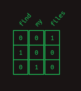
a symbol is an array of mostly zeros, vocab-length, with a single 1. each array element is a slot; the position of the one is the word’s identity.
markov chains
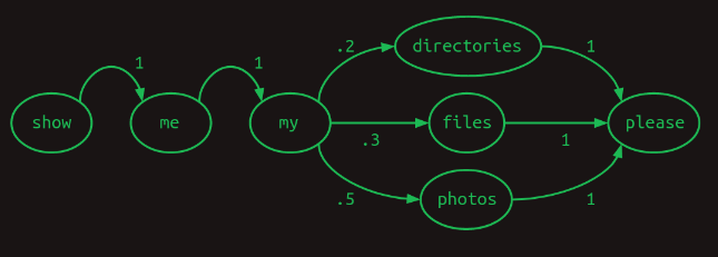
a chain satisfies the markov property: next-word probabilities depend only on recent words - first-order means the single most recent word (two words back would be second-order). in matrix form, rows and columns are both indexed by vocabulary words; pick the row of your current word, read probabilities off its columns. every element sits in [0, 1] and every row sums to 1.
first-order sequence model
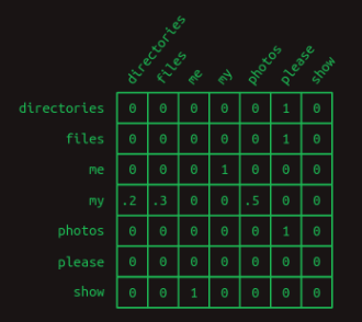
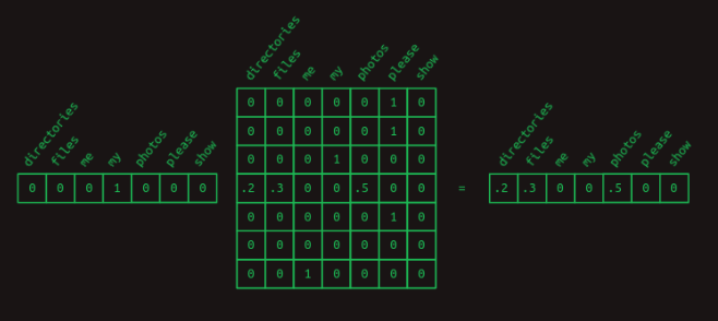
in a toy corpus of three sentences, almost all transition probabilities are 0 or 1 - branching happens in exactly one place (after “my”: directories, files, photos). and the neat trick, worth internalizing because attention will reuse it: multiplying a one-hot vector by the transition matrix pulls out one row - the next-word distribution of that word alone.
second-order sequence model
predicting from one word is like continuing a tune after one note. with two words:
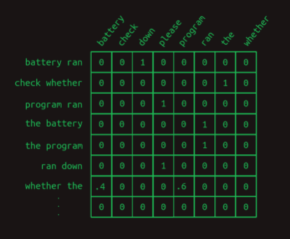
the cost is size: a separate row per word combination, so N² rows for vocabulary N. what it buys is confidence - more ones, fewer fractions, one branch left. more context for the next-word guess.
second-order with skips
two sentences that differ only by which word appeared 8 tokens back:
check the program log and find out whether it ran down please. check the battery log and find out whether it ran down please.
to know what comes after “ran” you must look 8 words back. an eighth-order model has N^8 rows - brute-force nonsense. the sly move: keep the model second-order, but take the most recent word paired with each word that came before. still two words per row, but now it reaches back for long-range dependencies - discarding most word-order information and keeping the powerful part.
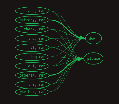
in matrix form:
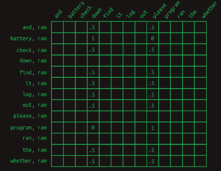
two things change, and both matter. first, predicting after “ran” no longer reads one row but a whole set of them - we’ve left the markov realm. each row is no longer the state of the sequence at one point; it’s one of many features that may describe the sequence at a point. and the matrix values stop being probabilities and become votes, summed to decide. second: most features are useless (every word appears in both sentences and adds nothing - stuck at 0.5). the exceptions do all the work: feature battery, ran votes 1 for “down” and 0 for “please”; feature program, ran votes the opposite. the presence of those two specific words earlier in the sentence is what decides.
selective masking = attention
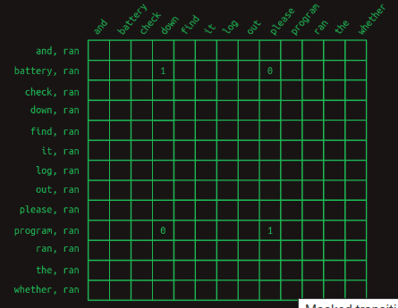
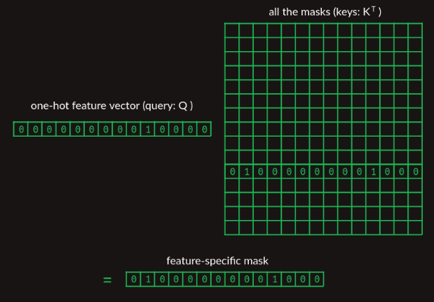
mask out the unhelpful features (“ran has a dependence on either program, ran or battery, ran - everything else can go”) and the predictions harden from a 25-percentage-point difference to certainty: a difference of “infinity percent”. there is no doubt what word comes next.
this process of selective masking is the attention called out in the title of the original paper - and that framing, down-weighting the irrelevant rows until the relevant ones dominate, is my favorite way to explain attention to someone who’s never seen it.
a state aside, since the KV-cache is often described as “a representation of the whole dataset the model is trained on” or a database of transformer state - that’s wrong: during generation, the cache stores the per-position key and value tensors of the current context so each new token doesn’t re-run attention over the whole prefix from scratch. the full mechanics still deserve their own note - todo below.
the feedforward block
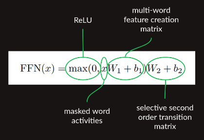
the sequence of feature-creation matrix multiplication → ReLU nonlinearity → transition-matrix multiplication is the feedforward processing applied after attention; paper equation 2 writes it compactly:
embeddings
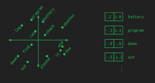
- a good embedding groups similar meanings together, and a model learning in that space generalizes automatically across the neighborhood: whatever it learns about one word applies to the words right next to it, which cuts the training data needed. (this is the word2vec intuition, formalized into the model’s own parameter space.)
- the trade: fewer embedded dimensions = fewer parameters = more information discarded. a language still needs room for its concepts to not step on each other. pick the embedding size to trade compute for accuracy.
attention mechanism
self-attention creates a matrix comparing each token with every token before it, weights set by pairwise relevance.
the part i had to have spelled out: each attention head maps a query word into yet another lower-dimensional embedded space, so attention becomes a relationship between word groups - it leans on semantic similarity (closeness in embed space) to generalize what it learned about similar words.
scaling: dividing every element by $\sqrt{d_k}$ keeps magnitudes from growing wildly and keeps backprop healthy.
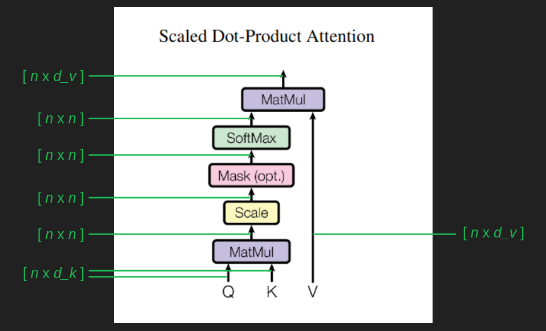
in this form the [n x n] attention matrix maps each element to the elements it should watch for the most relevant context. used as a filter over the values matrix $V$, it leaves only the attended values - which is the polite version of “ignores most of what came before and spotlights what matters”.
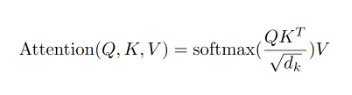
one humbling thing to remember: these calculations run for every element of the input, not just the latest word - for earlier words too (throwaway, their outputs are already decided) and for future words (unused for now, but there are indirect paths through which they affect the latest token’s attention, so they’re all computed; we just discard most of them when word probabilities are read off at the end).
q, k, v
- the query: the main representation of the word being re-represented (the “main word”)
- the key: the representation of all words as they’re being compared against the main word
- the value: the representation of all words - main word included - used to produce the main word’s final embedding

the attention layer returns one vector z per word: “what this word means contextualized against all others”.
the shapes version (attention arithmetic with seq_len = 20, embed_size = 128)
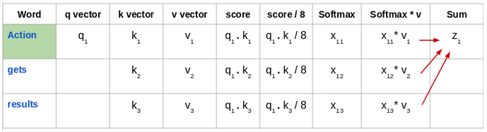
- input:
(20, 128). q, k, v all come out(20, 128)- same embed size as input is convenient, not mandatory. - scores:
q · kᵀ=(20, 128) · (128, 20)=(20, 20)- one score per word pair. - scale (numerical stability only: big values are unpleasant in deep nets), then softmax per row: each main word’s 20 scores now sum to 1.
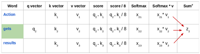
- weighted sum of values with the scores as weights: read row $i$ of the
(20, 20)matrix, use its 20 scalars to mix the 20(1, 128)value vectors → one contextualized(1, 128)embedding for word $i$. do it 20 times →(20, 128).
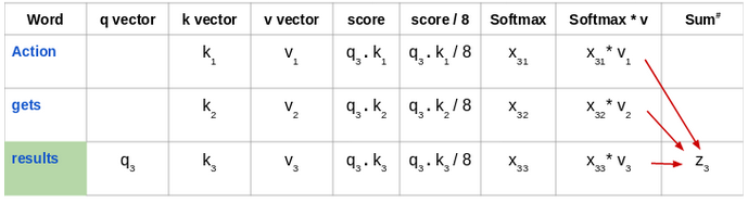
(despite the “it’s basically a cosine sim” shorthand i used to reach for: the scores are plain dot products of learned projections, no norm division of the two vectors, no cosine geometry - just scaled, softmaxed similarity the model trains to mean “attend here”.) the softmax inside is the same function the kernel notes optimize.
multi-head attention
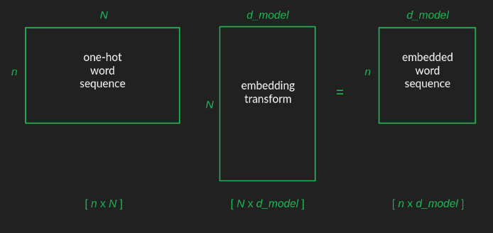
the paper’s knobs: $N$ vocabulary size (13 in the toy example; tens of thousands in practice), $n$ max sequence length (12 in the toy; a few hundred “in the paper - they don’t specify”; 2048 in GPT-3), $d_{model}$ 512, $d_k = d_v$ 64, $h = 8$ heads.
input matrix: stack one-hot row vectors → shape n x N.
why multiple heads? the nice version of the argument: attention isn’t binary 0/1 - softmax maps scores into [0, 1] and emphasizes the top value while squashing the rest (that’s the whole softmax trick. but the same mechanism robs us: a softmax-heavy attention tends to focus on a single element, and sometimes several preceding words should stay in mind together. the fix is heads: several attention instances run at once so the model considers several previous words simultaneously. the cost concern - head count multiplies the already-dominant attention compute - is answered by projecting into the lower-dim per-head space (shrunk matrices, cheap day saved).
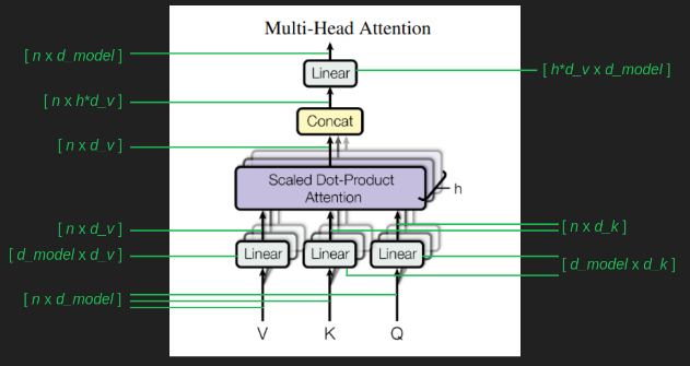
mechanics: each head’s output has the same shape as $V$; concatenate the $h$ results into one [n x h·dv] matrix, then transform with [h·dv x d_model] to land back at the input shape.
the shapes walkthrough of the split: 8 heads cut the 128-dim embedding into (8 heads, 16 per-head). sequence length 20 → (20, 8, 16); batch 128 → (128, 20, 8, 16). for the score computation swap dims 2/3: q becomes (128, 8, 20, 16), kᵀ is (128, 8, 16, 20), scores land at (128, 8, 20, 20) - 8 heads, 8 attention maps. each head ends with a 16-dim vector; concatenate 8 of them → 128 again. the point of the multiplicity: no single word always dominates - 8 softmaxed “smoothed” possibilities, where one head can give two words 0.45 each and zero the rest, in general it leans toward one.
add & norm
skip connections serve the gradient first. attention is a filter that blocks most of what tries to pass through, so small input changes can die in blocked channels - flat spots and ridges that trip up backpropagation. the skip adds a copy of the inputs to the output: even if every attention weight were zero, small input changes still produce noticeable output changes, so gradient descent doesn’t stall far from good solutions.
two nice framings worth keeping: the block enhances the raw embedding rather than recreating it (it learns to change the original representation, and everything trains so the sum makes sense); and the conveyor-belt view of stacked layers - each block pulls inputs off the line, computes, and puts whatever came out (useful or not) back on the belt.
layer norm: shift the matrix values to zero mean, scale to unit standard deviation. the batch-vs-layer norm distinction in one breath: 100 objects with 10 values each - batch norm normalizes 10 times across 100 objects (row-wise), layer norm normalizes 100 times across 10 values (column-wise). in a transformer we permanently compare representations within one sequence, so layer norm is the fit.
multiple layers
one attention layer = one path to good parameters: fragile, brittle, needs a lucky initialization. multiple layers, each consuming the previous one’s output, with skips, tolerate individual blocks failing - if one goes off the rails, a downstream block gets another chance to close the gap. the paper showed more layers help, with improvement going marginal past 6.
the encoder stack upgrade: sequence completion becomes translation. training needs source and matching target sequence; the full source runs through the encoder unmasked (we see the whole sentence before translating) and the final encoder output feeds every decoder layer as an input.
cross-attention = self-attention where $K$ and $V$ come from the final encoder output rather than the previous decoder layer; $Q$ still comes from the decoder side. this is the channel through which source-sequence information steers the target’s creation. and since the same embedded source reaches every decoder layer, successive layers are redundant backups cooperating on one task.
time-mixing vs channel-mixing
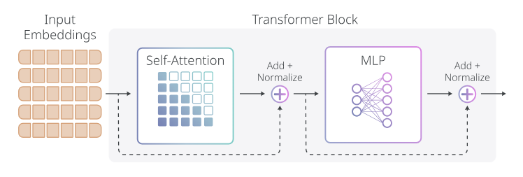
the input to each block is (sequence_length, hidden_size) - call them time dimension and channel dimension. every operation broadly falls into: mix along channels (1), mix along time (2), or both (3). self-attention is category 3 - the query projection mixes channels, the attention scores mix time - which abstracts a transformer block to a time-mixing op followed by a channel-mixing op. (this framing is exactly the hook MLLA’s linear-attention reform hangs its “attention is just a channel-mixer in disguise” argument on.)
context, retrieval, and what the transformer can’t do
transformers use context as short-term memory recalled with near-perfect fidelity - hence in-context learning: induction heads solving indirect object identification, or in-context linear regression straight from the papers’ examples.
and the flip side: the transformer doesn’t filter its context until recall time. so anything we suspect is useful gets filtered outside the model - with classic information retrieval machinery - and stuffed into the prompt: RAG. a human with a search engine is kind of a RAG system: you still need to know what to search, but whatever comes back is as salient as short-term memory.
breadcrumbs
- bahdanau attention - where the score-normalize-weighted-sum core was born, four years earlier
- bert - the same machinery with the mask flipped (bidirectional vs causal)
- rope - the positional-information half this note never covered (the walkthrough above quietly assumes positions exist somewhere)
- mlla - the linear-attention reformulation of everything in the multi-head section
- information retrieval - the filtering half of the RAG coda
- kl divergence - entropy and the softmax-adjacent math the attention scores lean on
papers & sources
- attention is all you need: https://arxiv.org/abs/1706.03762
- the walkthroughs merged above: e2eml.school/transformers, annotated transformer, hyugen-ai’s shapes walkthrough (link above), analytics vidhya 2019 primer
- video: the AIAYN explained playlist, the krish naik-style full course, karpathy’s build-along, mamba explained (thegradient)
- code: hkproj/pytorch-transformer
todos
- positional encodings are the conspicuous hole above - the walkthrough never writes them; fill alongside RoPE notes when redoing them together.
- my KV-cache correction is one paragraph of assertion; write the actual walkthrough (per-token state, why it’s $O(n^2)$ attention saved to $O(n)$ per new token) and link it here.
- derive the $\sqrt{d_k}$ scale properly (the variance argument from §3.2.1) instead of the “keeps magitudes from growing wildly” hand-wave above.
- re-read the annotated transformer end-to-end - it’s been queued forever and i’ve only ever used it as a reference dip.
- the flattened-transformer/MLLA linear-attention line: fold the focused-linear-attention math into mlla notes and cross-link here, so the “attention as time+channel mixing” section has its reformulation sibling.